Spline Interpolation

In both Polynomial Interpolation and Hermite Interpolation, we constructed a single, global polynomial covering the entire domain $[a, b]$.

Global polynomials suffer from a fundamental architectural flaw: global stiffness. Because a polynomial of degree $n$ is defined by a single formula, perturbing a single data point sends ripples across the entire interval. Furthermore, as the number of data points grows into hundreds or thousands, global polynomials become computationally ill-conditioned.

The modern resolution is piecewise approximation: partition the domain $[a, b]$ into smaller subintervals, fit a low-degree polynomial on each piece, and glue them together smoothly at the knots.

This note develops the theory of piecewise interpolation and cubic splines [1][1] R. L. Burden and J. D. Faires, Numerical Analysis, 9th ed. Brooks/Cole, Cengage Learning, 2011., [2][2] M. U. School of Mathematics, “MTH2051: Introduction to Computational Mathematics: Course Lecture Notes and Study Workbooks,” 2026. Monash University course materials and study workbooks, Semester 2, 2026.:

1. Piecewise Linear Interpolation: Proving the sharp $\frac{h^2}{8} \max |f''|$ error bound;
2. Piecewise Quadratic Interpolation: Matching midpoints for $\mathcal{O}(h^3)$ local accuracy;
3. Cubic Splines: Balancing $C^2$ smoothness against degrees of freedom;
4. Boundary Conditions: Contrasting Natural, Clamped, and Not-a-knot conditions, and the second-order boundary error qualification;
5. The Tridiagonal System: Deriving the three-moment equation and solving it in $\mathcal{O}(n)$ time;
6. Method Comparison: A comprehensive decision map for interpolation techniques.

Piecewise linear interpolation

The simplest piecewise method connects adjacent data points with straight line segments.

DefinitionPiecewise linear interpolant

Let $a = x_0 < x_1 < \dots < x_n = b$ partition $[a, b]$ into $n$ subintervals. On each subinterval $[x_i, x_{i+1}]$, the linear interpolant is

$$L_i(x) = f(x_i) \frac{x_{i+1} - x}{x_{i+1} - x_i} + f(x_{i+1}) \frac{x - x_i}{x_{i+1} - x_i}.$$

The global piecewise linear interpolant $L(x)$ is defined by $L(x) = L_i(x)$ for $x \in [x_i, x_{i+1}]$.

At each shared knot $x_i$, the adjacent pieces agree in value: $L_{i-1}(x_i) = f(x_i) = L_i(x_i)$. Therefore $L \in C^0([a, b])$. However, the slopes $L'_{i-1}$ and $L'_i$ generally differ, so $L$ has sharp corners and does not belong to $C^1([a, b])$.

The sharp uniform error bound

LemmaMaximum of the nodal quadratic factor

Let $[x_i, x_{i+1}]$ have length $h_i = x_{i+1} - x_i$. The quadratic function $q(x) = (x - x_i)(x_{i+1} - x)$ satisfies

$$\max_{x \in [x_i, x_{i+1}]} |(x - x_i)(x_{i+1} - x)| = \frac{h_i^2}{4},$$

attained uniquely at the midpoint $x_m = \frac{x_i + x_{i+1}}{2}$.

Proof

Expanding $q(x) = -x^2 + (x_i + x_{i+1})x - x_i x_{i+1}$, its derivative is $q'(x) = -2x + (x_i + x_{i+1})$. Setting $q'(x) = 0$ locates the unique critical point at $x_m = (x_i + x_{i+1})/2$.

Since $q''(x) = -2 < 0$, $q$ is concave down, and its maximum value is:

$$q(x_m) = (x_m - x_i)(x_{i+1} - x_m) = \left( \frac{h_i}{2} \right) \left( \frac{h_i}{2} \right) = \frac{h_i^2}{4}.$$

Because $q(x_i) = q(x_{i+1}) = 0$ at the endpoints, the maximum on $[x_i, x_{i+1}]$ is exactly $h_i^2 / 4$.

TheoremPiecewise linear error bound

Let $f \in C^2([a, b])$ and let $h = \max_i (x_{i+1} - x_i)$ be the maximum step size. Then

$$\max_{x \in [a, b]} |f(x) - L(x)| \le \frac{h^2}{8} \max_{t \in [a, b]} |f''(t)|.$$

Proof

On each subinterval $[x_i, x_{i+1}]$, the Cauchy interpolation error formula for $n = 1$ states that for each $x \in [x_i, x_{i+1}]$, there exists $\xi_x \in (x_i, x_{i+1})$ such that

$$f(x) - L_i(x) = \frac{f''(\xi_x)}{2} (x - x_i)(x - x_{i+1}).$$

Taking absolute values and applying Lemma 1:

$$|f(x) - L_i(x)| \le \frac{1}{2} \left( \max_{t \in [x_i, x_{i+1}]} |f''(t)| \right) \left( \frac{h_i^2}{4} \right) = \frac{h_i^2}{8} \max_{t \in [x_i, x_{i+1}]} |f''(t)|.$$

Taking the maximum over all subintervals $i = 0, \dots, n-1$ yields the global bound.

A crude bound that bounds $|x - x_i| \le h_i$ and $|x - x_{i+1}| \le h_i$ independently would yield $h^2 / 2$. Utilizing the parabola vertex sharpens the leading constant from $1/2$ to $1/8$, making the bound four times tighter. The convergence rate is second-order: halving the mesh size reduces the error by a factor of four.

Piecewise quadratic interpolation

To achieve higher accuracy, we can construct a quadratic polynomial on each subinterval $[x_i, x_{i+1}]$ by evaluating $f$ at the midpoint $m_i = (x_i + x_{i+1})/2$ in addition to the endpoints:

$$(x_i, f(x_i)), \quad (m_i, f(m_i)), \quad (x_{i+1}, f(x_{i+1})).$$

On each subinterval, this is a 3-node Lagrange interpolation problem. If $f \in C^3$, the local error has the form

$$f(x) - Q_i(x) = \frac{f^{(3)}(\xi)}{3!} (x - x_i)(x - m_i)(x - x_{i+1}),$$

yielding third-order convergence $\mathcal{O}(h_i^3)$.

However, adjacent quadratic pieces still fail to match in slope at the knots $x_i$: $Q'_{i-1}(x_i) \neq Q'_i(x_i)$. The curve remains non-differentiable at the knots.

Cubic splines

To eliminate slope and curvature discontinuities without increasing the polynomial degree to global heights, we turn to cubic splines.

The term spline originally referred to a flexible wooden strip used by shipbuilders and draftsmen, pinned down at discrete points with lead weights (called ducks) to trace fair, naturally smooth curves. Mechanically, the strip bends to minimize strain energy, producing a continuous second derivative across all joints.

DefinitionCubic spline interpolant

Let $a = x_0 < x_1 < \dots < x_n = b$. A function $S(x)$ is a cubic spline interpolant for $f$ through the data $(x_i, f(x_i))$ if:

1. Piecewise Cubic: On each subinterval $[x_i, x_{i+1}]$, $S(x) = S_i(x)$ is a polynomial of degree at most $3$;
2. Interpolation: $S(x_i) = f(x_i)$ for all $i = 0, 1, \dots, n$;
3. $C^2$ Smoothness: $S(x)$, $S'(x)$, and $S''(x)$ are continuous across the entire interval $[a, b]$.

Counting constraints and degrees of freedom

Let us determine whether a cubic spline is uniquely determined:

• There are $n$ subintervals, each carrying a cubic polynomial $S_i(x) = a_i + b_i x + c_i x^2 + d_i x^3$;
• Each cubic polynomial has $4$ coefficients, giving $4n$ total unknowns;
• Endpoint values on each piece: Matching the given data at both ends of each subinterval requires $S_i(x_i) = y_i$ and $S_i(x_{i+1}) = y_{i+1}$ for each $i = 0, \dots, n-1$, contributing $2n$ equations;
• First derivative continuity: Matching $S'_{i-1}(x_i) = S'_i(x_i)$ at the $n-1$ interior knots contributes $n-1$ equations;
• Second derivative continuity: Matching $S''_{i-1}(x_i) = S''_i(x_i)$ at the $n-1$ interior knots contributes $n-1$ equations.

Summing all continuity and interpolation conditions:

$$2n + (n - 1) + (n - 1) = 4n - 2.$$

Subtracting from the $4n$ degrees of freedom leaves:

$$4n - (4n - 2) = 2 \text{ degrees of freedom remaining}.$$

To specify the spline uniquely, we must supply exactly two additional boundary conditions.

Spline boundary conditions

Three standard boundary specifications are used in numerical practice:

DefinitionSpline boundary conditions

1. Natural (Free) Boundary Conditions:

$$S''(x_0) = 0 \quad \text{and} \quad S''(x_n) = 0.$$

The curvature is forced to zero at the boundary endpoints, mimicking a physical beam with free ends. 2. Clamped (Complete) Boundary Conditions:

$$S'(x_0) = f'(x_0) \quad \text{and} \quad S'(x_n) = f'(x_n).$$

The boundary slopes are clamped to match the true derivative of $f$. 3. Not-a-Knot Boundary Conditions:

$$S'''(x) \text{ is continuous across } x_1 \text{ and } x_{n-1}.$$

This forces $S_0(x) \equiv S_1(x)$ and $S_{n-2}(x) \equiv S_{n-1}(x)$, so $x_1$ and $x_{n-1}$ cease to be active knots (requiring $n \ge 3$).

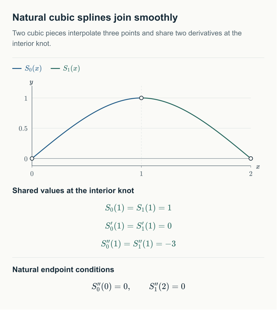
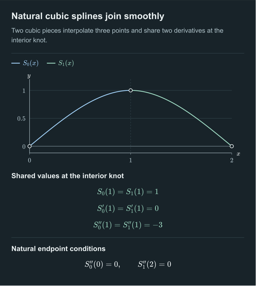
Accuracy qualification: the boundary curvature trap

Textbooks frequently state that cubic splines converge at fourth order: $\mathcal{O}(h^4)$. While true for clamped splines and not-a-knot splines on refining uniform meshes, this does not hold universally for natural splines.

If $f \in C^4([a, b])$, clamped boundary conditions guarantee

$$\max_{x \in [a, b]} |f(x) - S(x)| \le C h^4 \max_{t \in [a, b]} |f^{(4)}(t)|.$$

However, natural boundary conditions force $S''(a) = S''(b) = 0$. If the true function has non-zero boundary curvature ($f''(a) \neq 0$ or $f''(b) \neq 0$), the spline suffers from boundary curvature incompatibility.

Consider $f(x) = x^2$ on $[0, 1]$. Here $f^{(4)}(x) \equiv 0$, yet the natural spline cannot reproduce $x^2$ because $S''(0) = S''(1) = 0 \neq 2$. As a consequence, the global error rate of a natural spline degrades to second order:

$$\max_{x \in [a, b]} |f(x) - S_{\text{natural}}(x)| = \mathcal{O}(h^2).$$

Fourth-order convergence is restored for natural splines only if the true function naturally satisfies $f''(a) = f''(b) = 0$.

Derivation of the tridiagonal system

To compute the spline efficiently, we do not solve for the $4n$ polynomial coefficients directly. Instead, we express each cubic piece in terms of its second derivatives at the knots:

$$M_i = S''(x_i), \quad i = 0, 1, \dots, n.$$

Since each $S_i(x)$ is cubic, its second derivative $S''_i(x)$ is linear on $[x_i, x_{i+1}]$. Since $S''_i(x_i) = M_i$ and $S''_i(x_{i+1}) = M_{i+1}$, the linear Lagrange interpolant gives

$$S''_i(x) = M_i \frac{x_{i+1} - x}{h_i} + M_{i+1} \frac{x - x_i}{h_i}, \quad h_i = x_{i+1} - x_i.$$

Integrating $S''_i(x)$ twice and using the interpolation conditions $S_i(x_i) = y_i$ and $S_i(x_{i+1}) = y_{i+1}$ yields the closed-form expression:

$$S_i(x) = M_i \frac{(x_{i+1} - x)^3}{6 h_i} + M_{i+1} \frac{(x - x_i)^3}{6 h_i} + \left( y_i - \frac{M_i h_i^2}{6} \right) \frac{x_{i+1} - x}{h_i} + \left( y_{i+1} - \frac{M_{i+1} h_i^2}{6} \right) \frac{x - x_i}{h_i}.$$

By construction, this formula guarantees $C^0$ value interpolation and $C^2$ second-derivative continuity. It remains only to enforce $C^1$ first-derivative continuity at each interior knot:

$$S'_{i-1}(x_i) = S'_i(x_i), \quad i = 1, 2, \dots, n - 1.$$

Differentiating $S_i(x)$ and equating the one-sided limits at $x_i$ produces the celebrated Three-Moment Equation:

TheoremTridiagonal spline system

For $i = 1, 2, \dots, n - 1$, the knot second derivatives $M_i = S''(x_i)$ satisfy

$$h_{i-1} M_{i-1} + 2(h_{i-1} + h_i) M_i + h_i M_{i+1} = 6 \left( \frac{y_{i+1} - y_i}{h_i} - \frac{y_i - y_{i-1}}{h_{i-1}} \right).$$

For natural boundary conditions, setting $M_0 = M_n = 0$ reduces this to a square linear system of size $(n-1) \times (n-1)$ for the interior unknowns $M_1, \dots, M_{n-1}$:

$$\begin{bmatrix} 2(h_0 + h_1) & h_1 & 0 & \dots & 0 \\ h_1 & 2(h_1 + h_2) & h_2 & \dots & 0 \\ 0 & h_2 & 2(h_2 + h_3) & \dots & 0 \\ \vdots & & \ddots & \ddots & \vdots \\ 0 & \dots & 0 & h_{n-2} & 2(h_{n-2} + h_{n-1}) \end{bmatrix} \begin{bmatrix} M_1 \\ M_2 \\ M_3 \\ \vdots \\ M_{n-1} \end{bmatrix} = \begin{bmatrix} d_1 \\ d_2 \\ d_3 \\ \vdots \\ d_{n-1} \end{bmatrix}.$$

Notice that for every row $i$:

$$2(h_{i-1} + h_i) > h_{i-1} + h_i.$$

The coefficient matrix is strictly diagonally dominant and symmetric positive-definite. By the Gershgorin circle theorem, it is non-singular and well-conditioned.

Furthermore, because the matrix is tridiagonal, it can be solved using the Thomas algorithm (tridiagonal Gaussian elimination) in $\mathcal{O}(n)$ time and $\mathcal{O}(n)$ storage.

RemarkAlignment with standard textbook coefficients

In standard reference texts such as Burden and Faires [1][1] R. L. Burden and J. D. Faires, Numerical Analysis, 9th ed. Brooks/Cole, Cengage Learning, 2011., each cubic piece is expanded about its left knot:

$$S_j(x) = a_j + b_j(x - x_j) + c_j(x - x_j)^2 + d_j(x - x_j)^3, \quad x \in [x_j, x_{j+1}].$$

Because $S''_j(x_j) = 2 c_j = M_j$, the second derivatives $M_j$ map directly to the textbook coefficients:

$$a_j = y_j, \quad c_j = \frac{M_j}{2}, \quad d_j = \frac{M_{j+1} - M_j}{6 h_j}, \quad b_j = \frac{y_{j+1} - y_j}{h_j} - \frac{2 M_j + M_{j+1}}{6} h_j.$$

Dividing the three-moment equation by $3$ yields the textbook's tridiagonal system for the unknown coefficients $c_j$.

This interactive figure needs JavaScript.

Method comparison

We can now summarize the interpolation methods developed across the curriculum in a comparative decision table:

Method	Prescribed Data	Degree Bound	Global Smoothness	Convergence Rate	Locality & Sensitivity
Lagrange / Newton	Values $f(x_i)$	$n$ (Global)	$C^\infty$	Varies (Runge divergence on uniform grids)	Non-local: moving one point affects the entire curve
Chebyshev	Values at Chebyshev roots	$n$ (Global)	$C^\infty$	Geometric / Spectral for analytic $f$	Non-local: requires freedom to select node locations
Hermite	Values $f(x_i)$ and slopes $f'(x_i)$	$2n + 1$ (Global)	$C^\infty$	$\mathcal{O}(h^{2n+2})$ locally	Non-local: matches tangents, but global degree grows
Piecewise Linear	Values $f(x_i)$	$1$ (Local)	$C^0$	$\mathcal{O}(h^2)$ with sharp constant $1/8$	Strictly Local: perturbation affects only adjacent pieces
Piecewise Quadratic	Values and midpoints	$2$ (Local)	$C^0$	$\mathcal{O}(h^3)$	Strictly Local: corners persist at knots
Cubic Spline (Clamped)	Values $f(x_i)$ and $2$ boundary slopes	$3$ (Local pieces)	$C^2$	$\mathcal{O}(h^4)$ uniformly	Locally damped: perturbation decays exponentially away from knot
Cubic Spline (Natural)	Values $f(x_i)$ and $S''(a)=S''(b)=0$	$3$ (Local pieces)	$C^2$	$\mathcal{O}(h^2)$ unless $f''=0$ at boundaries	Locally damped: zero endpoint curvature

By breaking the monopoly of high-degree global polynomials, cubic splines achieve the golden standard of scientific interpolation: optimal $C^2$ smoothness, linear $\mathcal{O}(n)$ computational complexity, and bounded local influence.

References

1. [1] R. L. Burden and J. D. Faires, Numerical Analysis, 9th ed. Brooks/Cole, Cengage Learning, 2011. a b
2. [2] M. U. School of Mathematics, “MTH2051: Introduction to Computational Mathematics: Course Lecture Notes and Study Workbooks,” 2026. Monash University course materials and study workbooks, Semester 2, 2026. ↩