Newton–Cotes quadrature

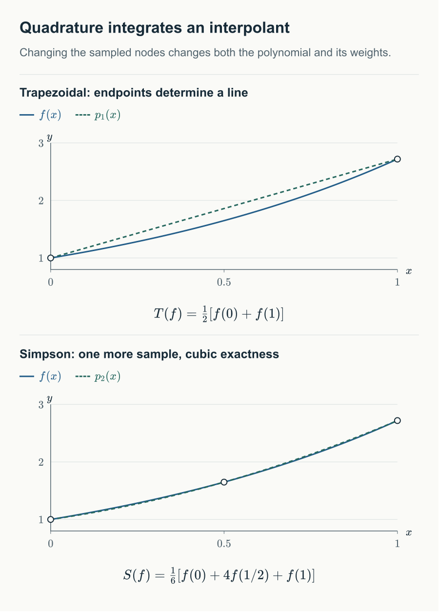
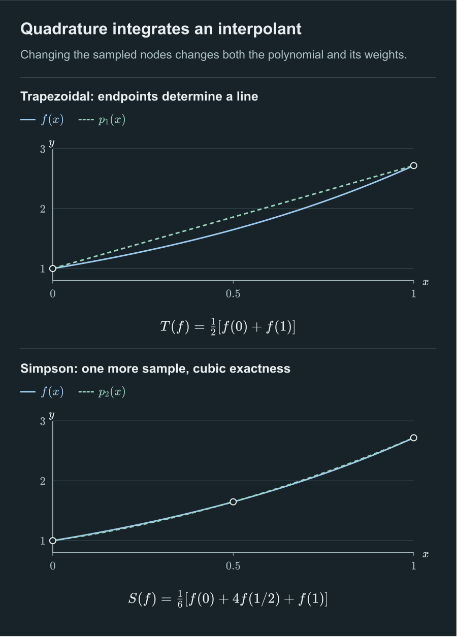
A quadrature rule replaces an integral with a weighted sum of finitely many function values. Newton–Cotes rules choose equally spaced nodes, interpolate, and integrate the polynomial. The nodes determine the weights; smoothness determines whether the error theorem applies.

Lecture note Sections 5.1–5.5 and 5.7 are the primary source. Write the exact integral as $I$, the approximation as $Q(f)$, and the signed error as exact minus approximate:

$$I=\int_a^b f(x)\,dx,\qquad E(f)=I-Q(f).$$

The interpolant uses the lecture note’s lowercase $p_n$. For general open rules we add the explicit indexing convention $x_0=a+h$, followed by equally spaced interior nodes. The workbook supplements the open two-point and Milne error derivations; their signs and constants are proved independently below [1][1] S. Rojas, “Lecture Notes on Computational Mathematics,” 2025. Course lecture note distributed with MTH2051; local source course-lecture-notes.pdf., [2][2] M. U. School of Mathematics, “MTH2051: Introduction to Computational Mathematics: Course Lecture Notes and Study Workbooks,” 2026. Monash University course materials and study workbooks, Semester 2, 2026., [3][3] R. L. Burden and J. D. Faires, Numerical Analysis, 9th ed. Brooks/Cole, Cengage Learning, 2011..

Interpolatory quadrature and degree of precision

DefinitionInterpolatory quadrature

For distinct nodes $x_0,\ldots,x_n$, form the Lagrange interpolant $p_n$ and define

$$Q(f)=\int_a^b p_n(x)\,dx =\sum_{i=0}^n w_i f(x_i),\qquad w_i=\int_a^b\ell_i(x)\,dx.$$

DefinitionDegree of precision

A rule has degree of precision $m$ if it is exact for every polynomial of degree at most $m$ and fails for at least one polynomial of degree $m+1$.

PropositionInterpolatory exactness

The rule above is exact for every polynomial of degree at most $n$.

Proof

Such a polynomial is its own unique interpolant. Equivalently, exactness through degree $m$ is the moment condition

$$\sum_iw_ix_i^k=\frac{b^{k+1}-a^{k+1}}{k+1},\qquad 0\leq k\leq m.$$

Necessity follows by taking monomials; sufficiency follows by linearity for their linear combinations.

A closed rule includes endpoints: $x_i=a+ih$, with $h=(b-a)/n$ and $n\geq1$. An open rule excludes them: $x_i=a+(i+1)h$, with $h=(b-a)/(n+2)$ and $n\geq0$. In both constructions, $n$ is the interpolation degree and there are $n+1$ nodes. The open spacing must not be confused with the closed spacing.

Deriving the common rules

Let $L=b-a$ and $m=(a+b)/2$. Integrating the basis polynomials gives trapezoidal and midpoint rules:

$$T(f)=\frac L2[f(a)+f(b)],\qquad M(f)=Lf(m).$$

The three-point closed rule is Simpson’s rule:

$$S(f)=\frac L6[f(a)+4f(m)+f(b)].$$

The open two-point rule uses the interior trisection points:

$$O_2(f)=\frac L2\left[f\!\left(a+\frac L3\right)+f\!\left(a+\frac{2L}3\right)\right].$$

Milne’s rule uses three interior quarter points:

$$O_3(f)=\frac L3\left[2f\!\left(a+\frac L4\right)-f(m)+2f\!\left(a+\frac{3L}4\right)\right].$$

ProofWeights and symmetry

Use coordinates centred at $m$. The two linear basis integrals in the trapezoidal and open two-point rules are equal and sum to $L$, so each weight is $L/2$. The midpoint rule integrates a constant basis, with weight $L$.

For Simpson’s nodes $-L/2,0,L/2$, the endpoint quadratic basis integrals are $L/6$ and the middle integral is $2L/3$. For Milne’s nodes $-L/4,0,L/4$, an outer basis is $s(s+L/4)/(2(L/4)^2)$, integrating to $2L/3$. The middle basis $1-s^2/(L/4)^2$ integrates to $-L/3$.

These quadratic interpolatory rules already integrate quadratics exactly. Symmetric nodes and weights also integrate every centred odd function to zero, including a centred cubic. Consequently Simpson and Milne integrate every cubic exactly.

Proving errors with an integrable remainder

A pointwise interpolation remainder involves $f^{(r)}(\xi_x)$. The unknown location changes with $x$ and need not vary continuously, so it cannot simply be taken outside the integral. An integral Taylor remainder avoids that difficulty.

TheoremPeano kernel representation

Let $f\in C^r[a,b]$ and suppose the linear error functional $E$ annihilates polynomials of degree below $r$. Then

$$E(f)=\int_a^b f^{(r)}(t)K_r(t)\,dt,$$$$K_r(t)=\frac{(b-t)^r}{r!} -\sum_iw_i\frac{(x_i-t)_+^{r-1}}{(r-1)!}, \qquad u_+=\max(u,0).$$

Proof

Repeated integration of the fundamental theorem of calculus gives

$$f(x)=\sum_{k=0}^{r-1}\frac{f^{(k)}(a)}{k!}(x-a)^k +\int_a^b f^{(r)}(t)\frac{(x-t)_+^{r-1}}{(r-1)!}\,dt.$$

Apply $E$. Its polynomial part vanishes. Interchange the integrals over the compact triangle $a\leq t\leq x\leq b$ and move the finite weighted sum inside the integral. The resulting factor is precisely $K_r$.

LemmaA kernel with one sign gives one remainder location

If $K_r$ has a fixed sign and a nonzero integral, there is $\xi\in[a,b]$ such that

$$E(f)=f^{(r)}(\xi)\int_a^bK_r(t)\,dt.$$

Proof

Bound the continuous derivative between its minimum and maximum, multiply by $|K_r|$, and integrate. Division by the positive integral of $|K_r|$ puts the weighted average between those extrema. The intermediate value theorem supplies $\xi$. Restore the sign if the kernel is negative. No continuity of an unknown remainder location is assumed.

For checking constants, scale each rule to the following reference interval. For symmetric rules and even remainder order, reflection about the midpoint makes the kernel symmetric, so a left-half expression suffices.

Rule and interval	Kernel on the left half	Integral over the whole interval
Trapezoidal, $[0,1]$, $r=2$	$t(t-1)/2$ on the whole interval	$-1/12$
Midpoint, $[0,1]$, $r=2$	$t^2/2$ for $0\leq t\leq1/2$	$1/24$
Open two-point, $[0,3]$, $r=2$	$t^2/2$; subtract $3(t-1)/2$ on $[1,3/2]$	$3/4$
Simpson, $[0,2]$, $r=4$	$t^3(3t-4)/72$ on $[0,1]$	$-1/90$
Milne, $[0,4]$, $r=4$	$t^4/24$; subtract $4(t-1)^3/9$ on $[1,2]$	$14/45$

Substitution into the kernel theorem gives these expressions; replacing $x$ by $a+b-x$ verifies reflection symmetry. Trapezoidal and Simpson kernels are nonpositive, and the midpoint kernel is nonnegative. The open two-point kernel on $[1,3/2]$ is $(t^2-3t+3)/2>0$. For Milne, $t^4/(t-1)^3$ decreases on $(1,2]$ to $16>32/3$, proving positivity there. Integrating the piecewise polynomials proves the constants rather than inferring them from examples.

TheoremSigned errors of five rules

Let $L=b-a$. Require $f\in C^2$ for the first three rules and $f\in C^4$ for the last two. Each row has its own remainder location $\xi$.

Rule	Degree of precision	$I-Q(f)$
Trapezoidal	1	$-L^3f''(\xi)/12$
Midpoint	1	$L^3f''(\xi)/24$
Open two-point	1	$L^3f''(\xi)/36$
Simpson	3	$-L^5f^{(4)}(\xi)/2880$
Milne	3	$7L^5f^{(4)}(\xi)/23040$

Proof

Use the kernel representation and the fixed-sign lemma. Affine scaling multiplies a second-order kernel integral by the cube of the scale and a fourth-order kernel integral by its fifth power. This gives all listed constants. A centred quadratic or quartic has a nonzero constant derivative and therefore a nonzero error. Combined with the established exactness, the degrees are exactly one or three.

On $[0,1]$, the open two-point error on $x^2$ is $1/18$, and Milne’s error on $x^4$ is $7/960$. These verify both signs and constants. Different rules generally have different $\xi$ values: a factor of two between constants does not imply that every pair of actual errors has that ratio.

The closed hierarchy: three-eighths and Boole

Week 7 also lists two higher-degree closed rules. Here $n$ remains the interpolation degree, $h=L/n$, and $f_i=f(a+ih)$:

$$S_{3/8}(f)=\frac{3h}{8}(f_0+3f_1+3f_2+f_3),\qquad n=3,$$ $$B(f)=\frac{2h}{45}(7f_0+32f_1+12f_2+32f_3+7f_4),\qquad n=4.$$

Integrating the corresponding Lagrange bases gives these weights. Substitution into the moment equations verifies exactness through degree three and five respectively. A symmetric closed rule with even interpolation degree $n$ gains at least one extra degree: interpolation covers through $n$, and the next centred monomial is odd, hence integrates and sums to zero. Odd $n$ has no such automatic extra guarantee.

TheoremThree-eighths and Boole errors

Require $f\in C^4$ for three-eighths and $f\in C^6$ for Boole. There are respective remainder locations with

$$I-S_{3/8}(f)=-\frac{3h^5}{80}f^{(4)}(\xi) =-\frac{L^5}{6480}f^{(4)}(\xi),$$$$I-B(f)=-\frac{8h^7}{945}f^{(6)}(\eta) =-\frac{L^7}{1935360}f^{(6)}(\eta).$$

Their degrees of precision are exactly three and five.

Proof

Use the proved Peano representation. On the reference interval $[0,3]$, the three-eighths fourth-order kernel on the left half is

$$K_4(t)=\frac{t^3(2t-3)}{48}-\frac3{16}(t-1)_+^3, \qquad0\leq t\leq\frac32.$$

Both terms are nonpositive; reflection covers the full interval. Piecewise integration gives $\int K_4=-3/80$.

For Boole on $[0,4]$, the sixth-order kernel on the left half is

$$K_6(t)=\frac{t^5(15t-28)-128(t-1)_+^5}{10800}, \qquad0\leq t\leq2.$$

It is nonpositive for $t\leq28/15$. On the remaining range use $F(t)=t^5(15t-28)/(t-1)^5$, whose derivative is

$$F'(t)=\frac{5t^4[3(t-3)^2+1]}{(t-1)^6}>0.$$

Thus $F(t)\leq F(2)=64<128$, proving the kernel is still nonpositive. Reflect and integrate to get $\int K_6=-8/945$. The fixed-sign lemma and scaling give the error formulas. Nonzero errors on quartic and sextic monomials, together with moment exactness, establish the exact degrees of precision.

Both rules are also available in the experiment. Higher-degree rules require higher regularity; extra nodes alone do not certify greater accuracy.

Experiment: what curve is integrated?

This interactive figure needs JavaScript.

Switch rules to compare their nodes, weights, and green interpolants. Milne’s negative weight is intentional. The square-root example can be evaluated by midpoint and open rules, but its endpoint derivatives do not satisfy the standard error hypotheses.

PropositionAmplification of sample perturbations

If each sampled value has perturbation at most $\delta$ in magnitude, the quadrature perturbation is at most $\delta\sum_i|w_i|$. This worst-case bound is attainable.

Proof

Apply the triangle inequality to the weighted perturbations. Choosing perturbation $\delta\operatorname{sign}(w_i)$ at node $i$ makes all contributions have the same sign and reaches the bound.

Positive weights give $\sum|w_i|=L$, whereas Milne gives $5L/3$. Increasing the degree of equally spaced interpolation is not automatically more reliable. A common alternative is to retain a low-degree rule and use composite quadrature on smaller panels.

References

1. [1] S. Rojas, “Lecture Notes on Computational Mathematics,” 2025. Course lecture note distributed with MTH2051; local source course-lecture-notes.pdf. ↩
2. [2] M. U. School of Mathematics, “MTH2051: Introduction to Computational Mathematics: Course Lecture Notes and Study Workbooks,” 2026. Monash University course materials and study workbooks, Semester 2, 2026. ↩
3. [3] R. L. Burden and J. D. Faires, Numerical Analysis, 9th ed. Brooks/Cole, Cengage Learning, 2011. ↩