Hermite Interpolation | Xingyu Yang

In Polynomial Interpolation, our interpolating polynomials were constrained solely by point values: $P_n(x_i) = y_i$ .

Yet in physical modelling, navigation, robotics, and fluid dynamics, sensors frequently measure velocities, momenta, or tangent directions alongside positional coordinates:

f(x_i) = y_i \quad \text{and} \quad f'(x_i) = y'_i.

If we apply standard point-value interpolation, the resulting curve passes through the points but may point in the wrong direction, introducing artificial undulations between the nodes.

Hermite interpolation incorporates derivative constraints directly into the polynomial space [1], [2]:

The Hermite Interpolation Problem: Formulating $2(n+1)$ simultaneous value and slope constraints in $P_{2n+1}$ ;
Existence and Uniqueness: Proving uniqueness via double roots and establishing bijectivity via rank-nullity;
The Decoupling Principle: Why squaring the Lagrange basis ( $\ell_i(x)^2$ ) eliminates value and slope cross-talk across nodes;
Error Remainder and Osculation: Proving the squared nodal error formula $\prod (x - x_i)^2$ and observing its quadratic contact geometry;
Newton Form with Confluent Nodes: Extending divided differences to repeated nodes and avoiding floating-point classification traps;
Incomplete Hermite and Osculating Interpolation: Transitioning from confluent limits toward Taylor expansions.

The Hermite interpolation problem

DefinitionHermite interpolating polynomial

Let $a < b$ , $f \in C^1([a, b])$ , and let $x_0, x_1, \dots, x_n$ be $n+1$ pairwise distinct nodes in $[a, b]$ . The Hermite interpolating polynomial is the polynomial $H_{2n+1} \in P_{2n+1}$ satisfying

H_{2n+1}(x_i) = f(x_i) \quad \text{and} \quad H'_{2n+1}(x_i) = f'(x_i) \quad \text{for each } i = 0, 1, \dots, n.

Here $P_m$ denotes the vector space of real polynomials of degree at most $m$ , with dimension $\dim(P_m) = m+1$ .

Counting conditions clarifies the required polynomial space:

There are $n+1$ nodes;
Each node supplies $2$ conditions (one function value, one first derivative);
The total number of prescribed data values is $N = 2(n+1) = 2n + 2$ ;
To guarantee that a generic linear system has a unique solution, the polynomial space must have dimension $2n + 2$ , which corresponds to degree at most $d = N - 1 = 2n + 1$ .

Existence and uniqueness

A condition count does not by itself prove that the resulting equations are linearly independent. The following double-root argument provides the proof.

TheoremExistence and uniqueness of the Hermite interpolant

Under the hypotheses of Definition 1, there exists exactly one polynomial $H_{2n+1} \in P_{2n+1}$ satisfying all $2n+2$ value and derivative conditions.

Proof

Uniqueness via root multiplicities. Suppose there exist two polynomials $H_1, H_2 \in P_{2n+1}$ satisfying the Hermite conditions:

H_1(x_i) = H_2(x_i) = f(x_i) \quad \text{and} \quad H'_1(x_i) = H'_2(x_i) = f'(x_i), \quad i = 0, 1, \dots, n.

Define the difference polynomial $Q(x) = H_1(x) - H_2(x)$ . Because $P_{2n+1}$ is a linear vector space, $Q \in P_{2n+1}$ , so either $Q \equiv 0$ or $\deg Q \le 2n+1$ .

Evaluate $Q$ and its derivative at each node $x_i$ :

\begin{aligned} Q(x_i) &= H_1(x_i) - H_2(x_i) = f(x_i) - f(x_i) = 0, \\ Q'(x_i) &= H'_1(x_i) - H'_2(x_i) = f'(x_i) - f'(x_i) = 0. \end{aligned}

In algebra, if a differentiable polynomial satisfies both $Q(x_i) = 0$ and $Q'(x_i) = 0$ , then $x_i$ is a root of multiplicity at least $2$ (a double root). By the factor theorem, $(x - x_i)^2$ divides $Q(x)$ .

Because the $n+1$ nodes $x_0, x_1, \dots, x_n$ are pairwise distinct, the quadratic factors $(x - x_0)^2, \dots, (x - x_n)^2$ are pairwise coprime. Therefore, their entire product divides $Q(x)$ :

\prod_{i=0}^n (x - x_i)^2 \;\Big|\; Q(x) \implies Q(x) = g(x) \prod_{i=0}^n (x - x_i)^2

for some polynomial $g(x)$ .

Now examine the degree:

The product factor has degree $\sum_{i=0}^n 2 = 2(n + 1) = 2n + 2$ ;
If $Q(x) \not\equiv 0$ , then $\deg Q = \deg g + (2n + 2) \ge 2n + 2$ ;
However, $Q \in P_{2n+1}$ requires $\deg Q \le 2n + 1$ .

Since $2n + 2 > 2n + 1$ , this is a direct contradiction. Hence $Q(x) \equiv 0$ for all $x \in \mathbb{R}$ , proving $H_1 = H_2$ .

Existence via linear algebra. Define the linear evaluation mapping

\mathcal{H}: P_{2n+1} \to \mathbb{R}^{2n+2}, \quad \mathcal{H}(p) = \Big( p(x_0), p'(x_0), p(x_1), p'(x_1), \dots, p(x_n), p'(x_n) \Big).

The uniqueness proof establishes that if $\mathcal{H}(p) = \mathbf{0}$ , then $p \equiv 0$ . Thus the kernel is trivial: $\ker(\mathcal{H}) = \{0\}$ , so $\mathcal{H}$ is injective.

Because $\dim(P_{2n+1}) = 2n + 2 = \dim(\mathbb{R}^{2n+2})$ , the Rank-Nullity Theorem guarantees that $\mathcal{H}$ is also surjective. Therefore $\mathcal{H}$ is bijective: every Hermite data vector has one and only one preimage in $P_{2n+1}$ , proving existence.

The decoupling principle and the Hermite basis

To construct $H_{2n+1}(x)$ constructively, we decompose the solution into a basis expansion:

H_{2n+1}(x) = \sum_{i=0}^n \Big( f(x_i) h_i(x) + f'(x_i) \hat{h}_i(x) \Big).

This requires two basis polynomials per node:

$h_i(x)$ : the value selector, matching function value $1$ at $x_i$ , with slope $0$ at $x_i$ , and vanishing (value and slope) at all foreign nodes;
$\hat{h}_i(x)$ : the slope selector, matching slope $1$ at $x_i$ , with value $0$ at $x_i$ , and vanishing (value and slope) at all foreign nodes.

Why linear Lagrange basis fails

Recall the standard Lagrange basis polynomial $\ell_i(x) = \prod_{j \neq i} \frac{x - x_j}{x_i - x_j} \in P_n$ . While $\ell_i(x_j) = 0$ for $j \neq i$ , its derivative $\ell'_i(x_j)$ is generally non-zero. Using $\ell_i(x)$ directly would create massive cross-talk between the derivative conditions across different nodes.

The squaring breakthrough

Consider the squared polynomial $\ell_i(x)^2 \in P_{2n}$ . By the chain rule:

\big(\ell_i^2\big)'(x) = 2 \ell_i(x) \ell'_i(x).

Evaluating at any foreign node $x_j$ ( $j \neq i$ ):

Value: $\ell_i(x_j)^2 = 0^2 = 0$ ;
Slope: $(\ell_i^2)'(x_j) = 2 \cdot 0 \cdot \ell'_i(x_j) = 0$ .

Squaring the Lagrange basis places an automatic double root at every foreign node $x_j$ ( $j \neq i$ ), silencing both value and slope cross-talk simultaneously.

Deriving the basis polynomials

Since $\ell_i(x)^2 \in P_{2n}$ , multiplying it by a linear polynomial $(A(x - x_i) + B)$ yields an element of $P_{2n+1}$ , providing two tunable parameters to calibrate the behavior at the home node $x_i$ .

DefinitionHermite basis functions

For each node $x_i$ ( $i = 0, \dots, n$ ), the Hermite basis polynomials are:

h_i(x) = \Big( 1 - 2\ell'_i(x_i)(x - x_i) \Big) \ell_i(x)^2, \quad \hat{h}_i(x) = (x - x_i) \ell_i(x)^2.

They satisfy the four Kronecker selector conditions:

h_i(x_j) = \delta_{ij}, \quad h'_i(x_j) = 0, \quad \hat{h}_i(x_j) = 0, \quad \hat{h}'_i(x_j) = \delta_{ij}.

Proof

Let $c_i = \ell'_i(x_i)$ .

Derivation of $h_i(x)$ : Let $h_i(x) = (A(x - x_i) + B)\ell_i(x)^2$ .
- Setting $h_i(x_i) = 1$ : with $\ell_i(x_i) = 1$ , we get $(A(0) + B)(1)^2 = B = 1$ .
- Differentiating: $h'_i(x) = A \ell_i(x)^2 + (A(x - x_i) + 1) \cdot 2\ell_i(x)\ell'_i(x)$ .
- Setting $h'_i(x_i) = 0$ : $A(1)^2 + (0 + 1) \cdot 2(1)(c_i) = A + 2c_i = 0 \implies A = -2c_i$ . Thus $h_i(x) = (1 - 2\ell'_i(x_i)(x - x_i))\ell_i(x)^2$ .
Derivation of $\hat{h}_i(x)$ : Let $\hat{h}_i(x) = (C(x - x_i) + D)\ell_i(x)^2$ .
- Setting $\hat{h}_i(x_i) = 0$ : $(C(0) + D)(1)^2 = D = 0$ .
- Differentiating: $\hat{h}'_i(x) = C \ell_i(x)^2 + C(x - x_i) \cdot 2\ell_i(x)\ell'_i(x)$ .
- Setting $\hat{h}'_i(x_i) = 1$ : $C(1)^2 + 0 = C = 1$ . Thus $\hat{h}_i(x) = (x - x_i)\ell_i(x)^2$ .

At foreign nodes $x_j$ ( $j \neq i$ ), $\ell_i(x_j) = 0$ and $\ell_i(x_j)^2 = 0$ , so both values and derivatives vanish identically.

Complete two-node worked example

ExampleTwo-node Hermite interpolant for sine on [0, 1]

Consider $f(x) = \sin(\pi x)$ on $[0, 1]$ with $n = 1$ (nodes $x_0 = 0$ and $x_1 = 1$ ).

Step 1: Node evaluations and slopes:

\begin{aligned} f(0) &= \sin(0) = 0, \quad f'(0) = \pi \cos(0) = \pi, \\ f(1) &= \sin(\pi) = 0, \quad f'(1) = \pi \cos(\pi) = -\pi. \end{aligned}

Step 2: Lagrange basis and derivatives:

\ell_0(x) = \frac{x - 1}{0 - 1} = 1 - x \implies \ell'_0(0) = -1, \quad \ell_1(x) = \frac{x - 0}{1 - 0} = x \implies \ell'_1(1) = 1.

Step 3: Hermite basis components:

At $x_0 = 0$ :

\begin{aligned} h_0(x) &= (1 - 2(-1)(x - 0))(1 - x)^2 = (1 + 2x)(1 - x)^2 = 1 - 3x^2 + 2x^3, \\ \hat{h}_0(x) &= (x - 0)(1 - x)^2 = x(1 - x)^2 = x - 2x^2 + x^3. \end{aligned}

At $x_1 = 1$ :

\begin{aligned} h_1(x) &= (1 - 2(1)(x - 1))x^2 = (3 - 2x)x^2 = 3x^2 - 2x^3, \\ \hat{h}_1(x) &= (x - 1)x^2 = x^3 - x^2. \end{aligned}

Step 4: Assembly of $H_3(x)$ :

\begin{aligned} H_3(x) &= f(0) h_0(x) + f'(0) \hat{h}_0(x) + f(1) h_1(x) + f'(1) \hat{h}_1(x) \\ &= 0 + \pi \hat{h}_0(x) + 0 - \pi \hat{h}_1(x) \\ &= \pi \Big( x(1 - x)^2 - x^2(x - 1) \Big) \\ &= \pi x(1 - x) \Big( (1 - x) - (-x) \Big) \\ &= \pi x (1 - x). \end{aligned}

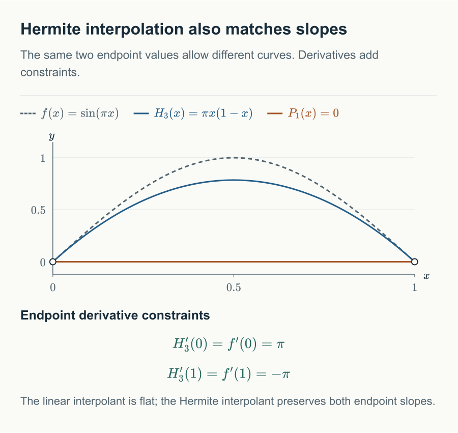
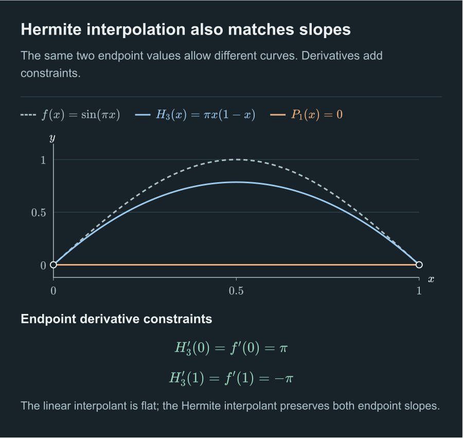
Notice that the cubic terms cancel out: the unique Hermite interpolant $H_3 \in P_3$ has actual degree $2$ .

Contrast this with the Lagrange linear interpolant $P_1(x)$ : because $f(0) = f(1) = 0$ , $P_1(x) \equiv 0$ , which completely misses the upward bulge of the sine wave. In contrast, Hermite interpolation matches the upward slope $\pi$ at $0$ and downward slope $-\pi$ at $1$ , capturing the crest accurately.

This interactive figure needs JavaScript.

Hermite cubic interpolant H3(x) matching sine values and endpoint slopes versus the flat linear interpolant P1(x).

Hermite error remainder formula

TheoremHermite error remainder formula

Let $a < b$ and $f \in C^{2n+2}([a, b])$ . Let $H_{2n+1} \in P_{2n+1}$ interpolate $f$ and $f'$ at the distinct nodes $x_0, \dots, x_n \in [a, b]$ . For each fixed $x \in [a, b]$ , there exists some intermediate point $\xi_x \in (a, b)$ such that

f(x) - H_{2n+1}(x) = \frac{f^{(2n+2)}(\xi_x)}{(2n+2)!} \prod_{i=0}^n (x - x_i)^2.

Proof

If $x$ is one of the nodes $x_i$ , both sides evaluate to zero.

Fix an arbitrary $x \in (a, b)$ with $x \neq x_i$ for all $i$ . Define the auxiliary function for $t \in [a, b]$ :

\omega(t) = \prod_{i=0}^n (t - x_i)^2, \quad K = \frac{f(x) - H_{2n+1}(x)}{\omega(x)}, \quad g(t) = f(t) - H_{2n+1}(t) - K \omega(t).

Observe the zeros of $g(t)$ :

At the evaluation point $t = x$ : $g(x) = 0$ by definition of $K$ ;
At each node $x_i$ : $g(x_i) = 0$ and $g'(x_i) = 0$ because both $f - H_{2n+1}$ and $\omega$ have double roots at $x_i$ .

Thus $g(t)$ has a double zero at each of the $n+1$ nodes and an additional simple zero at $x$ . Counting with multiplicity, $g(t)$ has at least $2(n+1) + 1 = 2n + 3$ zeros.

By repeated application of Rolle's theorem:

Differentiating $g(t)$ once leaves $n+1$ simple zeros at the nodes $x_i$ and produces $n+1$ additional zeros between adjacent distinct zeros, yielding at least $2n + 2$ zeros for $g'(t)$ ;
Repeating this process $2n + 2$ times proves that $g^{(2n+2)}$ has at least one interior zero $\xi_x \in (a, b)$ .

Now differentiate $g(t)$ exactly $2n + 2$ times:

$H_{2n+1}^{(2n+2)}(t) \equiv 0$ because $\deg H_{2n+1} \le 2n + 1$ ;
The polynomial $\omega(t) = t^{2n+2} + \mathcal{O}(t^{2n+1})$ is monic of degree $2n+2$ , so $\omega^{(2n+2)}(t) = (2n + 2)!$ .

Evaluating at $\xi_x$ :

g^{(2n+2)}(\xi_x) = f^{(2n+2)}(\xi_x) - 0 - K (2n + 2)! = 0 \implies K = \frac{f^{(2n+2)}(\xi_x)}{(2n + 2)!}.

Substituting $K$ back into $f(x) - H_{2n+1}(x) = K \omega(x)$ yields the formula.

Contact geometry: why squaring matters

Comparing the Lagrange and Hermite error formulas highlights a fundamental qualitative difference:

Lagrange Error: $\frac{f^{(n+1)}(\xi)}{(n+1)!} \prod (x - x_i)$ has simple zeros at the nodes. The error curve cuts straight through the horizontal axis at non-zero angle.
Hermite Error: $\frac{f^{(2n+2)}(\xi)}{(2n+2)!} \prod (x - x_i)^2$ has double zeros at the nodes. The error curve is tangent to the horizontal axis, touching it smoothly with quadratic flattening.

ExampleError estimation for the sine interpolant at x = 1/4

For $f(x) = \cos(\pi x) + x$ on $[0, 1]$ with $x_0 = 0, x_1 = 1$ , we have $f^{(4)}(x) = \pi^4 \cos(\pi x)$ , so $M_4 = \max |f^{(4)}| = \pi^4$ .

The theoretical error bound at $x = 1/4$ is:

|f(1/4) - H_3(1/4)| \le \frac{\pi^4}{24} (1/4)^2 (1 - 1/4)^2 = \frac{\pi^4}{24} \cdot \frac{1}{16} \cdot \frac{9}{16} = \frac{3\pi^4}{2048} \approx 0.1427.

Evaluating the true values: $f(1/4) = \cos(\pi/4) + 1/4 = \frac{\sqrt{2}}{2} + 0.25 \approx 0.9571$ , while the assembled polynomial gives $H_3(1/4) = 0.9375$ .

The true error is $E_{\text{true}} = |0.9571 - 0.9375| \approx 0.0196$ . The theoretical bound is a guaranteed upper bound, holding within a factor of roughly $7.3$ .

Newton form with confluent divided differences

Just as with Lagrange interpolation, assembling Hermite polynomials using basis functions requires $\mathcal{O}(n^2)$ effort when a new node is added. Can we construct Hermite polynomials using divided differences?

The limiting motivation

Recall the definition of the derivative:

\lim_{\varepsilon \to 0} \frac{f(x_i + \varepsilon) - f(x_i)}{\varepsilon} = f'(x_i).

If two distinct nodes coalesce to the same point, the ordinary divided difference converges to the derivative:

\lim_{x_{i+1} \to x_i} f[x_i, x_{i+1}] = f'(x_i).

This suggests repeating each node twice in the Newton table:

z_{2i} = z_{2i+1} = x_i, \quad i = 0, 1, \dots, n.

DefinitionConfluent divided differences

For the repeated node sequence $z_0, z_1, \dots, z_{2n+1}$ , the first-order divided difference is defined by

f[z_i, z_{i+1}] = \begin{cases} \frac{f(z_{i+1}) - f(z_i)}{z_{i+1} - z_i}, & \text{if } z_{i+1} \neq z_i, \\ f'(z_i), & \text{if } z_{i+1} = z_i. \end{cases}

Higher-order divided differences use the standard recursion whenever the outermost nodes are distinct:

f[z_i, \dots, z_{i+k}] = \frac{f[z_{i+1}, \dots, z_{i+k}] - f[z_i, \dots, z_{i+k-1}]}{z_{i+k} - z_i}.

TheoremHermite–Newton interpolation formula

With $z_0, z_1, \dots, z_{2n+1}$ denoting the repeated-node list, the Hermite interpolating polynomial is

H_{2n+1}(x) = f[z_0] + \sum_{k=1}^{2n+1} f[z_0, \dots, z_k] \prod_{j=0}^{k-1} (x - z_j).

Table reconstruction for the sine example

Let $x_0 = 0$ and $x_1 = 1$ , giving $z_0 = 0, z_1 = 0, z_2 = 1, z_3 = 1$ . The data values are $f(0) = 0, f'(0) = \pi, f(1) = 0, f'(1) = -\pi$ .

\begin{array}{c|c|cccc} k & z_k & f[z_k] & \text{1st order} & \text{2nd order} & \text{3rd order} \\ \hline 0 & 0 & \mathbf{0} & & & \\ 1 & 0 & 0 & \mathbf{\pi} \; (f'(0)) & & \\ 2 & 1 & 0 & \frac{0 - 0}{1 - 0} = 0 & \mathbf{\frac{0 - \pi}{1 - 0} = -\pi} & \\ 3 & 1 & 0 & -\pi \; (f'(1)) & \frac{-\pi - 0}{1 - 0} = -\pi & \mathbf{\frac{-\pi - (-\pi)}{1 - 0} = 0} \end{array}

Reading the top diagonal coefficients $c_0 = 0, c_1 = \pi, c_2 = -\pi, c_3 = 0$ :

\begin{aligned} H_3(x) &= 0 + \pi (x - 0) - \pi (x - 0)(x - 0) + 0 (x - 0)^2 (x - 1) \\ &= \pi x - \pi x^2 = \pi x (1 - x). \end{aligned}

The result matches the basis function expansion.

Numerical implementation caveat

In computational software, developers sometimes test whether two nodes are repeated using floating-point proximity: np.isclose(z[i], z[i+1]).

This is a dangerous numerical trap: two genuine distinct sample points separated by $10^{-8}$ will be falsely flagged as identical, replacing their legitimate divided difference with an unsupplied derivative.

In robust code, repeated nodes should be tracked using structural index parity (the pair index):

# Evaluate first-order differences by structural index parity
for i in range(2 * n + 1):
    if i % 2 == 0:
        Q[i, 1] = df_vals[i // 2]  # Exact derivative at repeated node
    else:
        Q[i, 1] = (Q[i + 1, 0] - Q[i, 0]) / (z[i + 1] - z[i])

Incomplete Hermite and osculating interpolation

What if the data does not specify first derivatives at every node?

For example, suppose we are given:

Value and slope at $x_1$ : $H(x_1) = f(x_1)$ , $H'(x_1) = f'(x_1)$ ;
Only value at $x_0$ : $H(x_0) = f(x_0)$ .

This supplies $N = 3$ conditions, which corresponds to the quadratic polynomial space $P_2$ .

Expanding $H \in P_2$ around $x_1$ :

H(x) = f(x_1) + f'(x_1)(x - x_1) + a_2 (x - x_1)^2.

Evaluating at $x_0$ yields the unique coefficient:

a_2 = \frac{f(x_0) - f(x_1) - f'(x_1)(x_0 - x_1)}{(x_0 - x_1)^2}.

Uniqueness follows from the fact that any difference polynomial $R(x)$ has root $(x - x_0)$ and double root $(x - x_1)^2$ . The divisor has degree $3$ , which contradicts $\deg R \le 2$ unless $R \equiv 0$ .

Transition to Taylor expansions

When all nodes coalesce to a single point $x_0$ , Hermite interpolation of orders $0, 1, \dots, m$ collapses into the classical Taylor polynomial:

T_m(x) = \sum_{k=0}^m \frac{f^{(k)}(x_0)}{k!} (x - x_0)^k.

Thus, Taylor polynomials are the single-point limit of osculating interpolation, while Lagrange polynomials are the simple-node limit. Hermite interpolation sits in the middle, blending spatial distribution with differential momentum.

From global Hermite to piecewise splines

While Hermite interpolation fixes tangent directions at each node, it remains a global polynomial method. As the number of nodes $n$ grows large, high-degree Hermite polynomials can still oscillate unacceptably away from the nodes.

In practical engineering, rather than raising the polynomial degree, we fix the degree to cubic and partition the domain into subintervals, matching values and derivatives locally.

In the next note, Spline Interpolation, we explore piecewise polynomials and derive $C^2$ natural cubic splines.

References

[1] R. L. Burden and J. D. Faires, Numerical Analysis, 9th ed. Brooks/Cole, Cengage Learning, 2011. ↩
[2] M. U. School of Mathematics, “MTH2051: Introduction to Computational Mathematics: Course Lecture Notes and Study Workbooks,” 2026. Monash University course materials and study workbooks, Semester 2, 2026. ↩

The Hermite interpolation problem

Existence and uniqueness

The decoupling principle and the Hermite basis

Why linear Lagrange basis fails

The squaring breakthrough

Deriving the basis polynomials

Complete two-node worked example

Hermite error remainder formula

Contact geometry: why squaring matters

Newton form with confluent divided differences

The limiting motivation

Table reconstruction for the sine example

Numerical implementation caveat

Incomplete Hermite and osculating interpolation

Transition to Taylor expansions

From global Hermite to piecewise splines

References

Comments