A single-panel rule approximates a whole interval by one low-degree polynomial. A composite rule partitions the interval and applies that same low-degree construction locally. Accuracy improves by refining the mesh instead of raising a global interpolation degree.
Use the convention in lecture note Section 5.6: is the number of small intervals and there are grid nodes:
Errors are always . We derive global constants from the single-panel theorem, keeping the grid width distinct from the Simpson panel width [1][1] S. Rojas, “Lecture Notes on Computational Mathematics,” 2025. Course lecture note distributed with MTH2051; local source course-lecture-notes.pdf., [2][2] M. U. School of Mathematics, “MTH2051: Introduction to Computational Mathematics: Course Lecture Notes and Study Workbooks,” 2026. Monash University course materials and study workbooks, Semester 2, 2026., [3][3] R. L. Burden and J. D. Faires, Numerical Analysis, 9th ed. Brooks/Cole, Cengage Learning, 2011..
Three composite rules
For , define
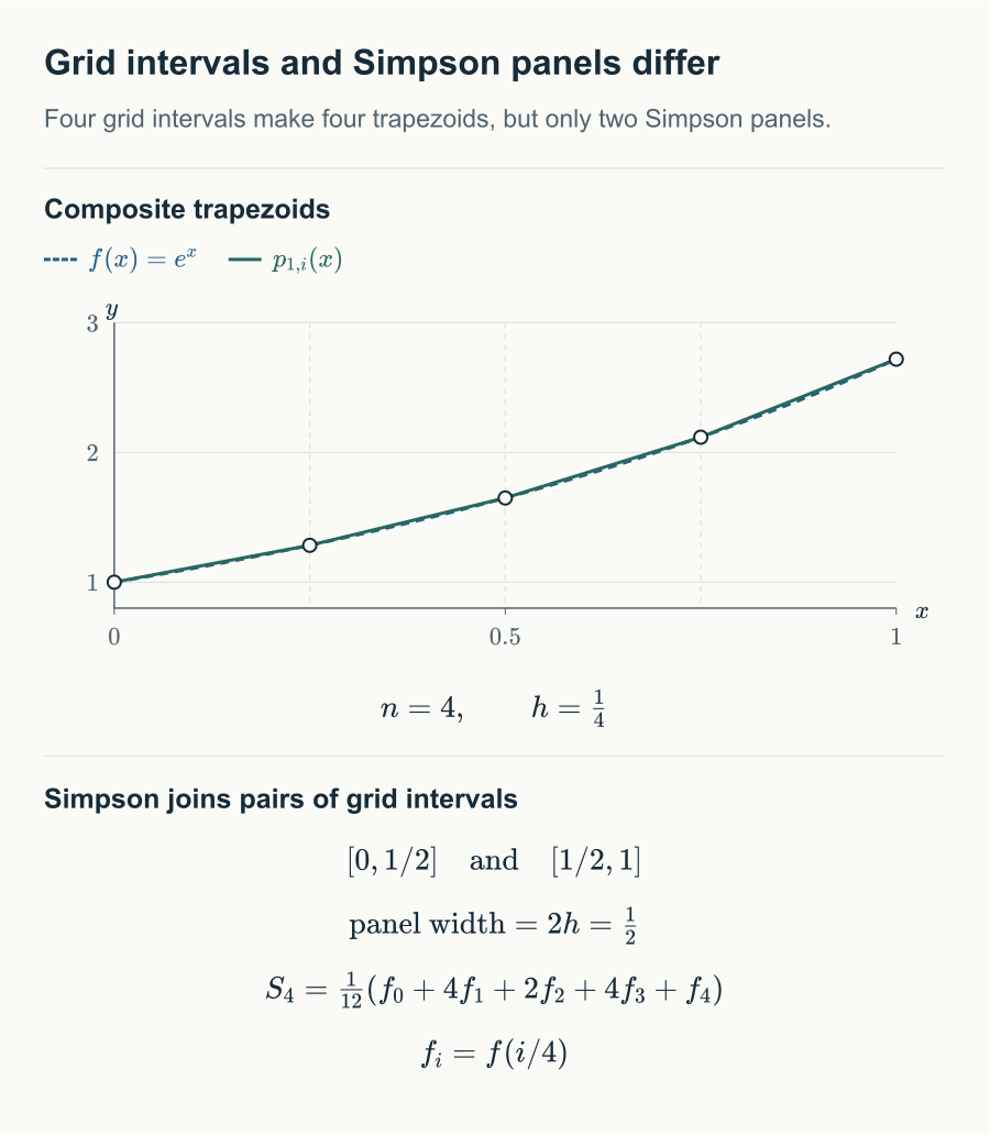
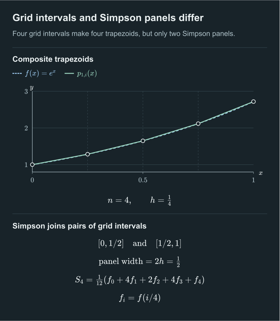
Require a positive even . Each Simpson panel covers two grid intervals and has width :
Sum the panel formulas. An interior trapezoidal node receives from each adjacent panel, giving total weight . Each Simpson panel has weights . Odd-index nodes are panel midpoints; even interior nodes join two panels; endpoints appear once. This yields the pattern . Each midpoint sample belongs to exactly one small interval.
From local to global error
For , there are points such that
For and even , there is with
Each trapezoidal panel has error . Sum the errors, identify the average of the derivative values with a value of the continuous derivative using the intermediate value theorem, and use . Midpoint panels have constant , giving their result in exactly the same way.
There are Simpson panels, each of width and error
Average their derivative values and sum the terms. The result is , as claimed.
Trapezoidal and midpoint rules have global order two, whereas Simpson has global order four. A local error is summed over order panels and becomes . Local and global orders cannot be interchanged. These orders describe bounds; a vanishing leading coefficient can give a higher observed order or exactness for a particular function.
Let
Replacing the remainder derivative by gives explicit bounds. A sufficient Simpson condition for tolerance is
Choose the smallest positive even integer at least . This requires an actual derivative bound; agreement between two computed meshes alone does not provide the same guarantee.
Convexity, bounds and cost
When , the error signs give . Convexity gives a direct proof too: on each panel the graph lies below its endpoint chord, so its integral lies below the trapezoid. The average of symmetric function values about the midpoint is at least the midpoint value; integrate that inequality to obtain the midpoint lower bound.
A direct evaluation requires function calls for trapezoidal, for midpoint, and for Simpson. Simpson requires an even . Comparing equal mesh counts and equal evaluation costs are distinct comparisons. Error constants involve derivatives of different orders, so there is no universal ranking for all integrands.
On a shared coarse mesh,
The fine trapezoidal mesh adds precisely the coarse-panel midpoints. Separating old and new nodes gives and . For , old interior nodes have weight , endpoints , and new midpoint nodes . These are the weights of . Substitute the first identity to obtain the final expression.
These are algebraic identities for arbitrary sampled values and need no smoothness. Their fourth-order error interpretation still requires the earlier hypotheses. The last identity is also the first Richardson extrapolation of trapezoidal values.
Observed order and failed smoothness
If the error has a nonzero leading term , then
Divide numerator and denominator by and take limits. The nonzero ensures a nonzero denominator eventually. A bound alone does not imply that the ratio tends to .
For , endpoint derivatives are unbounded, so neither the usual second-order nor fourth-order theorem applies. Avoiding endpoint samples does not restore smoothness. In fact its composite midpoint absolute error is : the first panel error is , and concavity makes all panel errors negative. For panel , the local second-derivative bound gives magnitude at most . Summing the convergent series gives an upper bound of the same order, while the nonzero first panel gives a lower bound.
Experiment and executable example
This interactive figure needs JavaScript.
Begin with the exponential to inspect error ratios, then switch to the square root to see smoothness fail. The narrow-peak example shows how small differences on coarse meshes can simply mean that the important region has not been sampled.
This implementation uses the same weights as the experiment, with counting small intervals:
def composite_simpson(f, a, b, n): if not isinstance(n, int) or not a < b or n < 2 or n % 2: raise ValueError("require a < b and positive even n") h = (b - a) / n total = f(a) + f(b) for i in range(1, n): total += (4 if i % 2 else 2) * f(a + i * h) return h * total / 3For on , the error is exactly , since the fourth derivative is constantly . This example simultaneously checks weights, error sign, and the definition of mesh width.
References
- [1] S. Rojas, “Lecture Notes on Computational Mathematics,” 2025. Course lecture note distributed with MTH2051; local source course-lecture-notes.pdf. ↩
- [2] M. U. School of Mathematics, “MTH2051: Introduction to Computational Mathematics: Course Lecture Notes and Study Workbooks,” 2026. Monash University course materials and study workbooks, Semester 2, 2026. ↩
- [3] R. L. Burden and J. D. Faires, Numerical Analysis, 9th ed. Brooks/Cole, Cengage Learning, 2011. ↩
Comments