Numerical differentiation

A derivative is a local rate of change, but a computer often receives only finitely many function values. Numerical differentiation chooses sample locations and weights, then asks how accurate that combination remains in finite precision.

Lecture note Sections 4.1–4.4 are the primary source: $h>0$ is the sample spacing; $D_{\mathrm{fwd}}(x;h)$, $D_{\mathrm{bwd}}(x;h)$, and $D_{\mathrm{cen}}(x;h)$ denote forward, backward, and centred differences. The second-derivative formula is $D^{(2)}(x;h)$. Every required sample must lie in the function’s domain. The basic difference names follow the lecture note; we add the argument $h$ to its $D_{\mathrm{fwd}}(x)$ and similar notation to expose step dependence. Labels such as $D_{3,\mathrm F}$ and $D_{5,\mathrm C}$ are auxiliary notation defined here. Workbooks and slides supply supplementary derivations and examples [1][1] S. Rojas, “Lecture Notes on Computational Mathematics,” 2025. Course lecture note distributed with MTH2051; local source course-lecture-notes.pdf., [2][2] M. U. School of Mathematics, “MTH2051: Introduction to Computational Mathematics: Course Lecture Notes and Study Workbooks,” 2026. Monash University course materials and study workbooks, Semester 2, 2026., [3][3] R. L. Burden and J. D. Faires, Numerical Analysis, 9th ed. Brooks/Cole, Cengage Learning, 2011..

Taylor’s theorem gives the basic formulas

DefinitionThree basic differences

Whenever the required samples exist, define

$$\begin{aligned} D_{\mathrm{fwd}}(x;h)&=\frac{f(x+h)-f(x)}h,\\ D_{\mathrm{bwd}}(x;h)&=\frac{f(x)-f(x-h)}h,\\ D_{\mathrm{cen}}(x;h)&=\frac{f(x+h)-f(x-h)}{2h}. \end{aligned}$$

TheoremSigned truncation errors

Assume $f\in C^2$ for the one-sided formulas and $f\in C^3$ for the centred formula. There are points in the respective sampling intervals such that

$$\begin{aligned} f'(x)-D_{\mathrm{fwd}}(x;h)&=-\frac h2 f''(\xi_F),\\ f'(x)-D_{\mathrm{bwd}}(x;h)&=\frac h2 f''(\xi_B),\\ f'(x)-D_{\mathrm{cen}}(x;h)&=-\frac{h^2}6 f'''(\xi_C). \end{aligned}$$

Proof

Taylor’s theorem with a Lagrange remainder gives

$$f(x+h)=f(x)+hf'(x)+\frac{h^2}{2}f''(\xi_F).$$

Rearrange and divide by $h$. Expanding $f(x-h)$ gives the backward formula; its linear term changes sign while its quadratic term does not.

For the centred formula, keep separate cubic remainders:

$$f(x\pm h)=f(x)\pm hf'(x)+\frac{h^2}{2}f''(x) \pm\frac{h^3}{6}f'''(\xi_\pm).$$

Subtracting cancels the even terms. The remainder contains the average of two values of $f'''$. Continuity and the intermediate value theorem identify this average with $f'''(\xi_C)$ at a point between them. Division by $2h$ proves the claim.

The basic one-sided formulas have accuracy order one; the centred formula has order two. Accuracy order and derivative order are different concepts. For a convex function, the forward formula overestimates the derivative and the backward formula underestimates it, directly from the signs above.

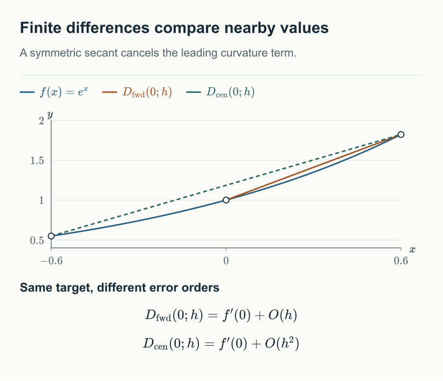
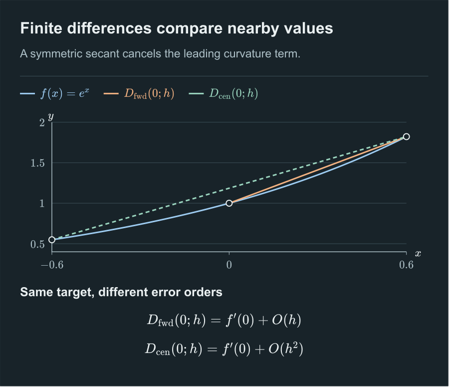
Differentiate an interpolating polynomial

Polynomial interpolation gives another construction: build $p_n$ through the samples and evaluate $p_n'(x_r)$. Following lecture note Section 5.1, lowercase $p_n$ denotes a general interpolating polynomial of degree at most $n$; uppercase $P_n$ is reserved for Legendre polynomials.

TheoremDerivative remainder at a node

Let $n\geq1$, let $x_0,\ldots,x_n$ be distinct, and assume $f\in C^{n+1}$ on their convex hull. Write

$$\omega(t)=\prod_{j=0}^n(t-x_j).$$

At any node $x_r$, there is a point $\xi$ in the node interval with

$$f'(x_r)-p_n'(x_r) =\frac{f^{(n+1)}(\xi)}{(n+1)!}\omega'(x_r).$$

Proof

Distinct nodes give $\omega'(x_r)\ne0$. Set

$$C=\frac{f'(x_r)-p_n'(x_r)}{\omega'(x_r)},\qquad \Phi(t)=f(t)-p_n(t)-C\omega(t).$$

All nodes are zeros of $\Phi$, and $\Phi'(x_r)=0$. There are at least $n+2$ zeros counting multiplicity. Repeated Rolle’s theorem gives $\Phi^{(n+1)}(\xi)=0$. Since $p_n^{(n+1)}=0$ and $\omega^{(n+1)}=(n+1)!$, the claimed value of $C$ follows.

This does not differentiate an unknown remainder location $\xi(t)$. Differentiating the pointwise interpolation remainder while treating that location as constant is invalid.

For nodes $x,x+h,x+2h$, the differentiated Lagrange weights at the left endpoint are $(-3,4,-1)/(2h)$:

$$D_{3,\mathrm F}(x;h) =\frac{-3f(x)+4f(x+h)-f(x+2h)}{2h}.$$

The nodal theorem gives

$$f'(x)-D_{3,\mathrm F}(x;h)=\frac{h^2}{3}f'''(\xi).$$

At the right endpoint use

$$D_{3,\mathrm B}(x;h) =\frac{3f(x)-4f(x-h)+f(x-2h)}{2h},$$

with the same signed remainder $h^2f'''(\xi)/3$. The three-point centred formula is $D_{\mathrm{cen}}(x;h)$; its middle sample has weight zero.

The five-point centred and forward formulas are

$$D_{5,\mathrm C}(x;h) =\frac{f(x-2h)-8f(x-h)+8f(x+h)-f(x+2h)}{12h},$$ $$D_{5,\mathrm F}(x;h) =\frac{-25f(x)+48f(x+h)-36f(x+2h)+16f(x+3h)-3f(x+4h)}{12h}.$$

For $f\in C^5$, their errors are

$$\begin{aligned} f'(x)-D_{5,\mathrm C}(x;h)&=\frac{h^4}{30}f^{(5)}(\xi),\\ f'(x)-D_{5,\mathrm F}(x;h)&=\frac{h^4}{5}f^{(5)}(\eta). \end{aligned}$$

The constants follow from $\omega'(x)=4h^4$ at the centred node and $24h^4$ at the forward endpoint, divided by $5!$. A backward five-point formula follows by replacing $h$ with $-h$ throughout the forward formula, including its denominator.

PropositionDerivation and uniqueness of the weights

These three- and five-point formulas are the derivatives of the corresponding Lagrange interpolants.

Proof

Write nodes as $x+r_jh$. Their basis polynomials satisfy

$$\ell_j(x+sh)=\prod_{k\ne j}\frac{s-r_k}{r_j-r_k}.$$

Differentiate with respect to $s$ and multiply by $1/h$ to obtain the weights. An independent check is polynomial reproduction: a formula $h^{-1}\sum_jw_jf(x+r_jh)$ must satisfy

$$\sum_jw_jr_j^k= \begin{cases}1,&k=1,\\0,&k=0,2,\ldots,n.\end{cases}$$

The three-point forward weights $(-3/2,2,-1/2)$ have moments $(0,1,0)$. The five-point centred weights $(1,-8,0,8,-1)/12$ and forward weights $(-25,48,-36,16,-3)/12$ both have moments $(0,1,0,0,0)$. Two weight vectors satisfying these conditions agree on every Lagrange basis polynomial, hence agree componentwise. This proves uniqueness.

Second derivatives and general moment conditions

Define

$$D^{(2)}(x;h)=\frac{f(x+h)-2f(x)+f(x-h)}{h^2}.$$

TheoremCentred second-derivative error

If $f\in C^4$, there is $\xi\in(x-h,x+h)$ such that

$$f''(x)-D^{(2)}(x;h)=-\frac{h^2}{12}f^{(4)}(\xi).$$

Proof

Expand each side through the cubic term, with fourth-order Lagrange remainders. Addition cancels the odd terms. Subtract $2f(x)$ and divide by $h^2$. The remainder is $h^2/12$ times an average of two fourth derivatives; continuity and the intermediate value theorem give the stated location.

Section 4.3 also gives the five-point centred second derivative. We introduce the auxiliary name $D_5^{(2)}$:

$$D_5^{(2)}(x;h)=\frac{-f(x+2h)+16f(x+h)-30f(x)+16f(x-h)-f(x-2h)}{12h^2}.$$

PropositionFourth-order five-point second derivative

For $f\in C^6$, as $h\to0$,

$$D_5^{(2)}(x;h)=f''(x)-\frac{h^4}{90}f^{(6)}(x)+o(h^4).$$

Proof

Offsets $(-2,-1,0,1,2)$ have weights $(-1,16,-30,16,-1)/12$. Their moments through degree five are $(0,0,2,0,0,0)$; the sixth moment is $-8$. Taylor expansion through degree six, divided by $h^2$, gives $f''$ and the term $-8h^4f^{(6)}(x)/6!=-h^4f^{(6)}(x)/90$. Continuity of the sixth derivative gives a remainder $o(h^4)$.

At a boundary, a four-point forward second-derivative formula is

$$\frac{2f(x)-5f(x+h)+4f(x+2h)-f(x+3h)}{h^2} =f''(x)-\frac{11}{12}h^2f^{(4)}(x)+O(h^3),$$

under $f\in C^5$. The weights $(2,-5,4,-1)$ have moments $(0,0,2,0)$ through degree three and moment $-22$ at degree four. Taylor substitution gives $-22/4!=-11/12$; the fifth-order remainder divided by $h^2$ is $O(h^3)$.

More generally, approximate an $r$th derivative with $h^{-r}\sum_jw_jf(x+r_jh)$. To achieve order $p$, match moments through degree $r+p-1$: only the degree-$r$ moment is nonzero, with value $r!$. Taylor’s theorem then gives an $O(h^p)$ error when the necessary derivatives are continuous and bounded. More samples alone do not guarantee higher accuracy.

Smaller steps can give larger errors

Following Section 4.4, $\epsilon_{\mathrm{mach}}$ denotes machine precision. Suppose each sampled value has absolute error at most $\delta$. The centred first derivative amplifies these perturbations by at most $\delta/h$. The centred second derivative has bound $4\delta/h^2$. These are sample-perturbation bounds; argument rounding and arithmetic introduce additional terms.

TheoremOptimal step in a first-derivative error model

For positive $C_1,C_2,\epsilon_{\mathrm{mach}}$ and $p\geq1$, the model

$$E_{\mathrm{model}}(h)=C_1h^p+\frac{C_2\epsilon_{\mathrm{mach}}}{h}$$

has a unique minimum for $h>0$, at

$$h_{\mathrm{opt}}=\left(\frac{C_2\epsilon_{\mathrm{mach}}}{pC_1}\right)^{1/(p+1)}.$$

Proof

The derivative is $pC_1h^{p-1}-C_2\epsilon_{\mathrm{mach}}/h^2$, with the sign of the strictly increasing expression $pC_1h^{p+1}-C_2\epsilon_{\mathrm{mach}}$. It crosses zero exactly once, from negative to positive. The model diverges at both ends, so this point is the unique global minimum. Substitution gives a minimum of order $\epsilon_{\mathrm{mach}}^{p/(p+1)}$, with constants depending on $C_1,C_2,p$.

For a second derivative, the perturbation term scales as $h^{-2}$, giving a model optimum proportional to $\epsilon_{\mathrm{mach}}^{1/(p+2)}$. The first-derivative scaling does not apply. Actual floating-point errors may oscillate or vanish accidentally; a U-shaped envelope is a trend model.

Experiment: truncation and rounding

This interactive figure needs JavaScript.

The experiment uses $f(x)=e^x$ at $x=0$, where both derivatives equal one. Halve a moderate step: forward error falls by roughly two, centred error by roughly four. Continue reducing the step and compare the measured error with the illustrative envelope. Switch to a second derivative to see stronger perturbation amplification.

Formula	Approximation at $h=0.1$	Absolute error from one
Forward	1.051709181	0.051709181
Centred	1.001667500	0.001667500
Five-point centred	0.999996663	0.000003337

These values check the derivation; they do not replace the error theorems. For measured data, also inspect noise and whether the sampling geometry matches the formula.

Choosing a formula

Start with a centred formula at an interior point when the function is smooth; use a one-sided formula at a boundary. Check sample availability before choosing accuracy order, then estimate derivative and noise scales. Richardson extrapolation can remove a leading error term under a suitable expansion. It cannot remove arbitrary measurement noise.

References

1. [1] S. Rojas, “Lecture Notes on Computational Mathematics,” 2025. Course lecture note distributed with MTH2051; local source course-lecture-notes.pdf. ↩
2. [2] M. U. School of Mathematics, “MTH2051: Introduction to Computational Mathematics: Course Lecture Notes and Study Workbooks,” 2026. Monash University course materials and study workbooks, Semester 2, 2026. ↩
3. [3] R. L. Burden and J. D. Faires, Numerical Analysis, 9th ed. Brooks/Cole, Cengage Learning, 2011. ↩