Adaptive Simpson integration

A uniform mesh spends the same effort everywhere, even when an integrand varies rapidly only in a small region. Adaptive integration estimates error locally and refines panels that have not yet met their assigned tolerance.

Lecture note Section 5.12 is the primary source. We use its $S(a,b)$, $S_2$, absolute error estimate $E$, and tolerance $\mathrm{tol}$. The difference $\Delta=S_2-S(a,b)$ and corrected value $Q_{\mathrm{corr}}$ are auxiliary notation defined here. The lecture algorithm accepts $S_2$; we also derive a Richardson correction and use that option in the experiment. An estimate is not a rigorous guarantee [1][1] S. Rojas, “Lecture Notes on Computational Mathematics,” 2025. Course lecture note distributed with MTH2051; local source course-lecture-notes.pdf., [2][2] M. U. School of Mathematics, “MTH2051: Introduction to Computational Mathematics: Course Lecture Notes and Study Workbooks,” 2026. Monash University course materials and study workbooks, Semester 2, 2026., [3][3] R. L. Burden and J. D. Faires, Numerical Analysis, 9th ed. Brooks/Cole, Cengage Learning, 2011..

Coarse panels, refined panels and fifteen

Let $m=(a+b)/2$ and $L=b-a$. The coarse Simpson value is

$$S(a,b)=\frac L6[f(a)+4f(m)+f(b)].$$

Bisect and define

$$S_2=S(a,m)+S(m,b),\qquad \Delta=S_2-S(a,b).$$

The coarse rule uses three samples; refinement adds two quarter-point samples.

TheoremLocal Richardson error estimate

For $f\in C^6$, on shrinking intervals with uniformly bounded relevant derivatives,

$$I-S_2=\frac{\Delta}{15}+O(L^7).$$

The corrected value

$$Q_{\mathrm{corr}}=S_2+\frac{\Delta}{15}$$

therefore has local error $O(L^7)$. Following the lecture note, $E=|\Delta|/15$ is a computed absolute error estimate, not the exact error.

Proof

Expand about the midpoint through degree five with remainder $O(L^6)$. Integration and Simpson agree through degree three; symmetry removes the fifth-degree term. The quartic term gives

$$I-S(a,b)=-\frac{L^5}{2880}f^{(4)}(m)+O(L^7).$$

Each half-panel contributes a term proportional to $(L/2)^5$. The average of the fourth derivatives at the two half-panel centres differs from $f^{(4)}(m)$ by $O(L^2)$, so

$$I-S_2=-\frac{L^5}{46080}f^{(4)}(m)+O(L^7).$$

Thus the coarse leading error is sixteen times the refined one. Subtract to obtain $\Delta=15(I-S_2)+O(L^7)$. Divide and correct. The stated seventh-order remainder uses $C^6$ regularity; the usual $C^4$ Simpson theorem alone does not imply this stronger remainder.

RemarkChecking the lecture note coefficient

Section 5.12 prints denominator $92160$ after adding the two half-panel errors. Since $2(L/2)^5/2880=L^5/46080$, the correct denominator is $46080$, giving a coarse-to-refined leading-error ratio of sixteen. We retain the lecture notation $S_2,E,\mathrm{tol}$ and use the coefficients and signs established above.

The denominator fifteen estimates the total error of the two refined Simpson panels. It is neither the error of one half-panel nor a strict bound for the corrected value. On meshes too coarse for the asymptotic model, it may miss important features.

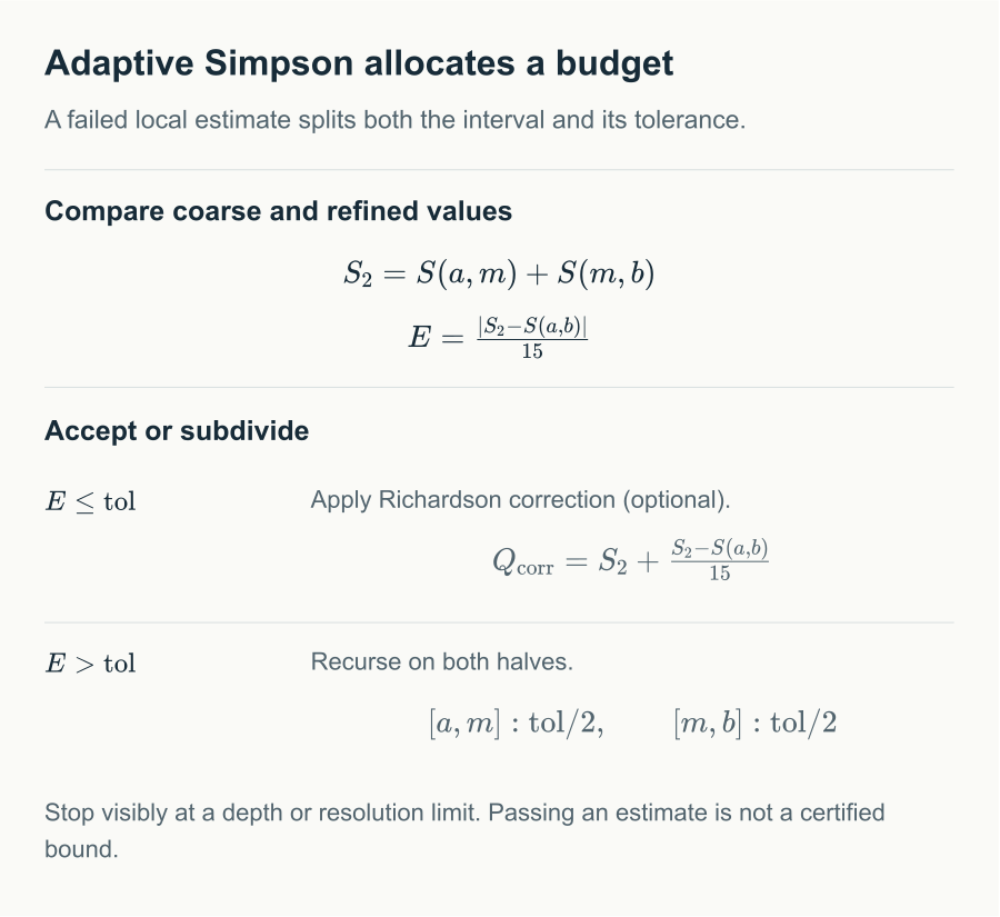
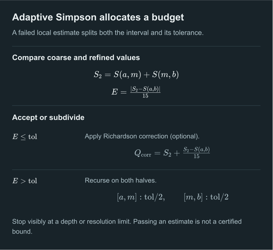
Allocate the tolerance

Assign a panel an absolute tolerance $\mathrm{tol}>0$. If $|\Delta|\leq15\mathrm{tol}$, accept the corrected value. Otherwise recurse on both halves, each with tolerance $\mathrm{tol}/2$.

PropositionConservation of tolerance budget

Starting from root tolerance $\mathrm{tol}$ and splitting each parent budget equally, the sum of all leaf budgets remains $\mathrm{tol}$.

Proof

Initially there is one budget $\mathrm{tol}$. A split replaces a number $u$ by $u/2+u/2$, preserving the sum. Induct on the number of splits.

If each leaf’s true error is at most its budget, the triangle inequality bounds total error by $\mathrm{tol}$. The algorithm checks only $E$, however, so budget conservation does not prove that the true errors satisfy those bounds.

With a proved local fourth-derivative bound $B_4$, the uncorrected refined value does satisfy

$$|I-S_2|\leq\frac{L^5B_4}{46080}.$$

Apply the single-panel theorem to each half and add. Such a derivative bound provides different evidence from a difference between two computed values.

Recursion and sample reuse

Algorithm 1 Adaptive Simpson recursion

Require: interval $[a,b]$, cached $f(a),f(m),f(b),S(a,b)$, tolerance $\mathrm{tol}$, remaining depth $d$

1:evaluate the two quarter points

2:$S_L\gets S(a,m)$ and $S_R\gets S(m,b)$

3:$\Delta\gets S_L+S_R-S(a,b)$

4:if $|\Delta|\leq15\mathrm{tol}$ then

5:return $(S_L+S_R+\Delta/15,\ \mathrm{accepted})$

6:end if

7:if $d=0$ then

8:return $(S_L+S_R+\Delta/15,\ \mathrm{limit})$

9:end if

10:recurse left with cached samples, tolerance $\mathrm{tol}/2$, depth $d-1$

11:recurse right with cached samples, tolerance $\mathrm{tol}/2$, depth $d-1$

12:return sum of child values and combined status

Acceptance means that the estimator test passed. A limit status means that the computation stopped before that test passed, and must not be reported as success. An implementation also needs to reject nonfinite function values and detect when floating-point resolution makes a midpoint or quarter point coincide with an endpoint.

The experiment caches samples and adds only two new function values per visited panel. With $N$ final leaves, the binary tree has $2N-1$ visited nodes; including the initial three samples gives $4N+1$ evaluations. The tree count follows because each split increases the leaf count by one and the total node count by two.

Experiment: local refinement and stopping

This interactive figure needs JavaScript.

Start with the smooth exponential, then choose a narrow peak. Adjust tolerance and compare leaf boundaries, function calls, summed estimates, and actual error. Set the maximum depth to zero to inspect the retained limit status.

The square root does not satisfy the endpoint smoothness hypotheses. The algorithm may still return a useful approximation, but the proof above does not explain all of its behaviour.

An estimator can miss the entire error

CounterexampleAll five initial samples vanish

On $[0,1]$, take

$$f(x)=\prod_{r=0}^4\left(x-\frac r4\right)^2.$$

All coarse and refined samples vanish, so $S=S_2=\Delta=0$. For any positive tolerance, the algorithm immediately accepts and returns zero, yet

$$\int_0^1f(x)\,dx=\frac5{1419264}>0.$$

Proof

The five sample locations are exactly the roots. The polynomial is nonnegative and strictly positive elsewhere, so its integral is positive. To check the exact constant, the unsquared product is

$$x^5-\frac52x^4+\frac{35}{16}x^3-\frac{25}{32}x^2+\frac3{32}x.$$

Square and integrate each monomial using $\int_0^1x^k\,dx=1/(k+1)$ to obtain the fraction. This is a smooth polynomial, demonstrating that smoothness alone does not make an initial coarse estimate trustworthy.

The experiment’s hidden-positive-polynomial preset is this example. Multiplying it by an arbitrary positive constant makes the true error arbitrarily large while all initial samples remain zero. Thus finitely many function samples, without further function-class restrictions or derivative bounds, cannot supply a universal certified integration error.

Interpreting the result

Keep the approximation, error estimate, evaluation count, and stopping status together. If discontinuities or peaks are known, split there before relying on recursive discovery. Use proved derivative bounds or interval methods when a certificate is required; for efficient approximation, compare different initial partitions and other rules.

The six chapters now connect local polynomial approximation to computation: differentiation and quadrature construct local formulas, composite rules accumulate panel errors, extrapolation cancels known powers, Gauss selects nodes by orthogonality, and adaptation allocates effort using local estimates. Each improvement has its own mathematical conditions.

Adaptive estimates for other rules

Section 5.12 also considers a general order-$p$ rule. Use auxiliary mesh labels $Q_0$ for the coarse value and $Q_2$ for the sum on two halves. If a common leading-error model gives $I-Q_0\approx2^p(I-Q_2)$, subtraction yields

$$I-Q_2\approx\frac{Q_2-Q_0}{2^p-1},\qquad E\approx\frac{|Q_2-Q_0|}{2^p-1}.$$

An $n$-point Gauss rule on each panel has composite order $p=2n$, giving denominator $2^{2n}-1$. Smoothness and the common leading-term model remain necessary; changing the quadrature rule does not turn a difference estimate into a true error bound.

References

1. [1] S. Rojas, “Lecture Notes on Computational Mathematics,” 2025. Course lecture note distributed with MTH2051; local source course-lecture-notes.pdf. ↩
2. [2] M. U. School of Mathematics, “MTH2051: Introduction to Computational Mathematics: Course Lecture Notes and Study Workbooks,” 2026. Monash University course materials and study workbooks, Semester 2, 2026. ↩
3. [3] R. L. Burden and J. D. Faires, Numerical Analysis, 9th ed. Brooks/Cole, Cengage Learning, 2011. ↩