Polynomial Interpolation

Connecting discrete observations to continuous reality is a foundational task in scientific computation. In physical experiments, telemetry streams, and numerical simulations, we rarely hold closed-form mathematical functions. Instead, we receive a finite set of sampled data points:

$$(x_0, y_0), (x_1, y_1), \dots, (x_n, y_n).$$

How do we construct a continuous model that passes exactly through each observation?

Polynomials are the primary algebraic candidate: they are infinitely differentiable, straightforward to integrate and differentiate analytically, and fast to evaluate on digital hardware using Horner's nested scheme.

This note establishes the core algebraic mechanics of polynomial interpolation [1][1] R. L. Burden and J. D. Faires, Numerical Analysis, 9th ed. Brooks/Cole, Cengage Learning, 2011., [2][2] M. U. School of Mathematics, “MTH2051: Introduction to Computational Mathematics: Course Lecture Notes and Study Workbooks,” 2026. Monash University course materials and study workbooks, Semester 2, 2026.:

1. The Interpolation Problem: Formulating exact matching in the polynomial vector space $P_n$;
2. Approximation versus Interpolation: Why Weierstrass's existential promise differs fundamentally from discrete interpolation;
3. The Lagrange Form: Building the interpolant using geometric selector switches ($\ell_i(x_j) = \delta_{ij}$);
4. Existence and Uniqueness: Establishing why $n+1$ distinct points define exactly one polynomial of degree at most $n$;
5. The Newton Divided-Difference Form: Constructing the interpolant incrementally so that new data points stream in at $\mathcal{O}(n)$ marginal cost.

The interpolation problem

DefinitionPolynomial interpolation

Given $n+1$ distinct real nodes $x_0, x_1, \dots, x_n$ and corresponding values $y_0, y_1, \dots, y_n$, a polynomial $P_n \in P_n$ is an interpolating polynomial if

$$P_n(x_i) = y_i, \quad i = 0, 1, \dots, n.$$

Here $P_n$ denotes the real vector space of all polynomials of degree at most $n$:

$$P_n = \left\{ \sum_{k=0}^n a_k x^k : a_k \in \mathbb{R} \right\}.$$

The space $P_n$ is parametrized by $n+1$ coefficients $a_0, a_1, \dots, a_n$, so its dimension is $\dim(P_n) = n+1$. Two distinct data points determine a straight line in $P_1$. Three non-collinear points determine a parabola in $P_2$. In general, matching $n+1$ scalar conditions requires an $(n+1)$-dimensional function space.

Approximation versus interpolation

Before constructing the polynomial, we must distinguish between two easily confused concepts: approximating a continuous function and interpolating discrete samples.

TheoremWeierstrass approximation theorem

Let $f \in C([a,b])$. For every tolerance $\varepsilon > 0$, there exists an integer $m \ge 0$ and a polynomial $q_m \in P_m$ such that

$$\max_{x \in [a,b]} |f(x) - q_m(x)| < \varepsilon.$$

The Weierstrass theorem provides an existential guarantee: continuous functions on compact intervals can be approximated uniformly by polynomials of sufficiently high degree.

However, Weierstrass does not claim that the unique polynomial interpolating $f$ at $n+1$ equally spaced sample points will converge to $f$ as $n \to \infty$. In fact, forcing a high-degree global polynomial through equidistant points can trigger catastrophic boundary divergence. The distinction is fundamental:

• Approximation asks for some polynomial that remains within an $\varepsilon$-tube across the entire interval $[a,b]$;
• Interpolation constructs the unique polynomial matching the function values at prescribed discrete nodes $x_0, \dots, x_n$.

This interactive figure needs JavaScript.

The Lagrange basis

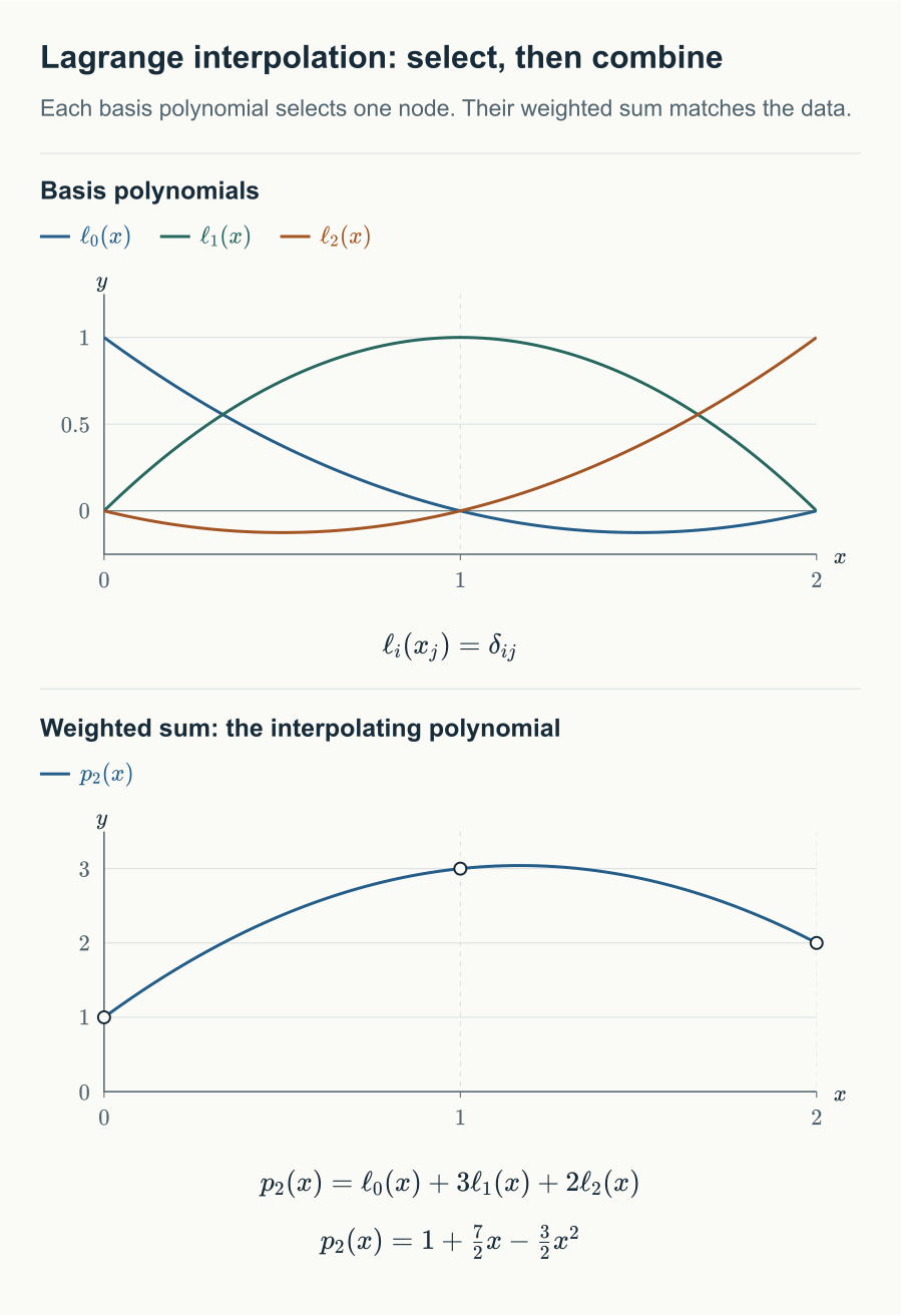
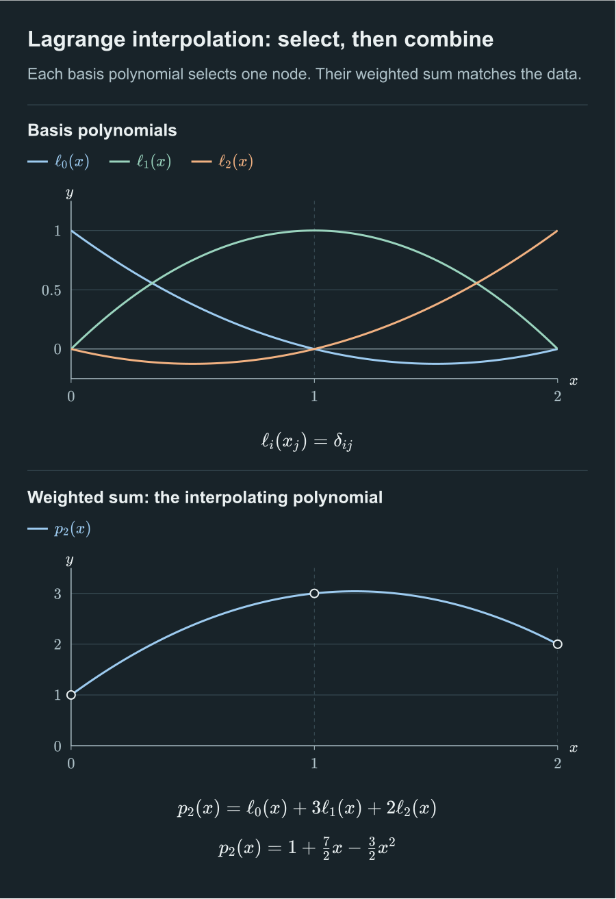
To construct the interpolating polynomial directly, we look for a basis of $P_n$ consisting of "selector switches": for each node $x_i$, we construct a basis polynomial $\ell_i(x)$ that evaluates to $1$ at $x_i$ and vanishes at all foreign nodes $x_j$ ($j \neq i$).

DefinitionLagrange basis polynomials

For $n+1$ pairwise distinct nodes $x_0, \dots, x_n$, the $i$-th Lagrange basis polynomial $\ell_i \in P_n$ is defined by

$$\ell_i(x) = \prod_{\substack{j=0 \\ j \neq i}}^n \frac{x - x_j}{x_i - x_j}.$$

It satisfies the Kronecker delta selector property:

$$\ell_i(x_j) = \delta_{ij} = \begin{cases} 1, & j = i, \\ 0, & j \neq i. \end{cases}$$

The algebraic design is direct:

1. The numerator $\prod_{j \neq i} (x - x_j)$ has degree $n$ and places a root at every node other than $x_i$;
2. The denominator $\prod_{j \neq i} (x_i - x_j)$ is a non-zero scalar constant that normalizes the value at $x = x_i$ to exactly $1$.

DefinitionLagrange interpolating polynomial

Given sample values $y_i = f(x_i)$, the Lagrange interpolating polynomial is

$$P_n(x) = \sum_{i=0}^n y_i \ell_i(x).$$

Evaluating $P_n(x)$ at any node $x_k$ isolates a single term:

$$P_n(x_k) = \sum_{i=0}^n y_i \ell_i(x_k) = \sum_{i=0}^n y_i \delta_{ik} = y_k.$$

Thus $P_n$ satisfies all $n+1$ interpolation conditions by construction.

ExampleQuadratic Lagrange interpolation for three points

Consider the data points $(0, 1)$, $(1, 3)$, and $(2, 2)$, with $n = 2$. The three quadratic basis polynomials are:

$$\begin{aligned} \ell_0(x) &= \frac{(x - 1)(x - 2)}{(0 - 1)(0 - 2)} = \frac{1}{2}(x - 1)(x - 2), \\ \ell_1(x) &= \frac{(x - 0)(x - 2)}{(1 - 0)(1 - 2)} = -x(x - 2), \\ \ell_2(x) &= \frac{(x - 0)(x - 1)}{(2 - 0)(2 - 1)} = \frac{1}{2}x(x - 1). \end{aligned}$$

Assembling the linear combination:

$$\begin{aligned} p_2(x) &= 1 \cdot \ell_0(x) + 3 \cdot \ell_1(x) + 2 \cdot \ell_2(x) \\ &= \frac{1}{2}(x^2 - 3x + 2) - 3(x^2 - 2x) + (x^2 - x) \\ &= -\frac{3}{2}x^2 + \frac{7}{2}x + 1. \end{aligned}$$

Checking the nodes: $p_2(0) = 1$, $p_2(1) = 3$, and $p_2(2) = 2$.

PropositionProperties of the Lagrange basis

The $n+1$ polynomials $\ell_0, \ell_1, \dots, \ell_n$:

1. Are linearly independent in $P_n$;
2. Form a basis for $P_n$;
3. Satisfy the partition of unity identity:

$$\sum_{i=0}^n \ell_i(x) = 1 \quad \text{for all } x \in \mathbb{R}.$$

Proof

To prove linear independence, suppose $\sum_{i=0}^n c_i \ell_i(x) = 0$ for all $x$. Evaluating this polynomial identity at $x = x_k$ yields

$$\sum_{i=0}^n c_i \ell_i(x_k) = \sum_{i=0}^n c_i \delta_{ik} = c_k = 0$$

for each $k = 0, 1, \dots, n$. Hence all coefficients vanish, establishing linear independence.

Since $\dim(P_n) = n+1$ and the collection contains $n+1$ linearly independent polynomials, it spans $P_n$ and forms a basis.

Finally, consider the constant function $f(x) \equiv 1 \in P_n$. Its unique interpolant in $P_n$ through the nodes is itself. Expanding it in the Lagrange basis gives $\sum_{i=0}^n 1 \cdot \ell_i(x) = 1$, which proves the partition of unity.

Existence and uniqueness

TheoremExistence and uniqueness of the interpolant

Let $x_0, x_1, \dots, x_n$ be $n+1$ pairwise distinct real numbers, and let $y_0, y_1, \dots, y_n$ be arbitrary real numbers. There exists exactly one polynomial $P_n \in P_n$ such that

$$P_n(x_i) = y_i, \quad i = 0, 1, \dots, n.$$

Proof

Existence. The Lagrange formula $P_n(x) = \sum_{i=0}^n y_i \ell_i(x)$ is a linear combination of elements of $P_n$, so $P_n \in P_n$. By the selector property, $P_n(x_i) = y_i$ for all $i$.

Uniqueness. Suppose $q_n \in P_n$ also satisfies $q_n(x_i) = y_i$ for $i = 0, 1, \dots, n$. Define the difference polynomial

$$r(x) = P_n(x) - q_n(x).$$

Since $P_n$ is a linear vector space, $r \in P_n$. Evaluating $r$ at each node:

$$r(x_i) = P_n(x_i) - q_n(x_i) = y_i - y_i = 0, \quad i = 0, 1, \dots, n.$$

Thus $r(x)$ has at least $n+1$ distinct roots. By the fundamental property of polynomials, a non-zero polynomial of degree at most $n$ can have at most $n$ roots. Therefore $r(x)$ must be the zero polynomial:

$$r(x) \equiv 0 \implies P_n(x) = q_n(x) \quad \text{for all } x \in \mathbb{R}.$$

The Newton divided-difference form

Although the Lagrange form offers an elegant closed-form proof of existence, it is computationally inefficient when data arrives incrementally. Adding a new sample point $(x_{n+1}, y_{n+1})$ alters the denominator and numerator of every basis polynomial $\ell_i(x)$, requiring an $\mathcal{O}(n^2)$ complete reconstruction.

The Newton form solves this by constructing the interpolant progressively:

$$P_k(x) = P_{k-1}(x) + a_k \prod_{j=0}^{k-1} (x - x_j).$$

Each new basis element $\prod_{j=0}^{k-1} (x - x_j)$ vanishes at all previous nodes $x_0, \dots, x_{k-1}$, preserving the values already matched and requiring only a single new coefficient $a_k$.

DefinitionDivided differences

Let $x_0, \dots, x_n$ be distinct nodes with values $f(x_0), \dots, f(x_n)$. The zeroth divided difference is

$$f[x_i] = f(x_i).$$

The first divided difference is

$$f[x_i, x_{i+1}] = \frac{f[x_{i+1}] - f[x_i]}{x_{i+1} - x_i}.$$

Higher-order divided differences are defined recursively for $k \ge 2$ by

$$f[x_i, x_{i+1}, \dots, x_{i+k}] = \frac{f[x_{i+1}, \dots, x_{i+k}] - f[x_i, \dots, x_{i+k-1}]}{x_{i+k} - x_i}.$$

The denominator of a $k$-th order divided difference is always the span between the two outermost nodes, $x_{i+k} - x_i$.

TheoremNewton form of the interpolating polynomial

The unique polynomial $P_n \in P_n$ interpolating $f$ at the distinct nodes $x_0, \dots, x_n$ can be expressed in Newton form as

$$P_n(x) = f[x_0] + \sum_{k=1}^n f[x_0, x_1, \dots, x_k] \prod_{j=0}^{k-1} (x - x_j).$$

Proof

Let $P_{0, k}(x)$ be the unique polynomial in $P_k$ interpolating $f$ at $x_0, \dots, x_k$. Consider the difference

$$P_{0, k}(x) - P_{0, k-1}(x).$$

Both polynomials match $f$ at $x_0, \dots, x_{k-1}$, so their difference has roots at each of these $k$ points. By the factor theorem:

$$P_{0, k}(x) - P_{0, k-1}(x) = c_k \prod_{j=0}^{k-1} (x - x_j),$$

where $c_k$ is the leading coefficient of $P_{0, k}(x)$.

Telescoping this relation from $k = 1$ to $n$ yields:

$$P_n(x) = P_{0, n}(x) = P_{0, 0}(x) + \sum_{k=1}^n c_k \prod_{j=0}^{k-1} (x - x_j).$$

It remains to identify $c_k$. Using the Neville recurrence relation:

$$P_{0, k}(x) = \frac{(x - x_0) P_{1, k}(x) - (x - x_k) P_{0, k-1}(x)}{x_k - x_0}.$$

Equating the coefficient of $x^k$ on both sides shows that the leading coefficient satisfies the exact divided-difference recurrence:

$$c_k = \frac{\operatorname{coeff}(P_{1, k}, x^{k-1}) - \operatorname{coeff}(P_{0, k-1}, x^{k-1})}{x_k - x_0}.$$

By induction on $k$, the leading coefficient of $P_{0, k}(x)$ is $f[x_0, \dots, x_k]$.

The divided-difference table

Divided differences are computed systematically in a triangular array:

$$\begin{array}{c|cccc} x_i & f[x_i] & \text{1st order} & \text{2nd order} & \text{3rd order} \\ \hline x_0 & \mathbf{f[x_0]} & & & \\ & & \mathbf{f[x_0, x_1]} & & \\ x_1 & f[x_1] & & \mathbf{f[x_0, x_1, x_2]} & \\ & & f[x_1, x_2] & & \mathbf{f[x_0, x_1, x_2, x_3]} \\ x_2 & f[x_2] & & f[x_1, x_2, x_3] & \\ & & f[x_2, x_3] & & \\ x_3 & f[x_3] & & & \end{array}$$

The Newton coefficients $a_k = f[x_0, \dots, x_k]$ are the bold entries along the top diagonal.

ExampleStep-by-step table construction and incremental update

Suppose we are given three initial observations: $(1, 2)$, $(2, 3)$, and $(4, 9)$.

1. Zeroth order: $f[x_0] = 2$, $f[x_1] = 3$, $f[x_2] = 9$.
2. First order:

$$f[x_0, x_1] = \frac{3 - 2}{2 - 1} = 1, \quad f[x_1, x_2] = \frac{9 - 3}{4 - 2} = 3.$$

3. Second order:

$$f[x_0, x_1, x_2] = \frac{3 - 1}{4 - 1} = \frac{2}{3}.$$

The quadratic interpolant is:

$$p_2(x) = 2 + 1 \cdot (x - 1) + \frac{2}{3}(x - 1)(x - 2).$$

Now suppose a fourth data point $(5, 12)$ arrives. We do not rebuild the table. We simply append the new row:

• $f[x_2, x_3] = \frac{12 - 9}{5 - 4} = 3$;
• $f[x_1, x_2, x_3] = \frac{3 - 3}{5 - 2} = 0$;
• $f[x_0, x_1, x_2, x_3] = \frac{0 - 2/3}{5 - 1} = -\frac{1}{6}$.

The updated cubic polynomial is obtained by adding a single term:

$$p_3(x) = p_2(x) - \frac{1}{6}(x - 1)(x - 2)(x - 4).$$

At the previous nodes $1, 2, 4$, the product factor vanishes, preserving the previously matched values automatically.

Horner nested evaluation

Expanding the Newton form into monomial powers $a x^2 + b x + c$ is numerically unstable and computationally wasteful. Instead, we evaluate the polynomial in nested Horner form:

$$P_n(x) = a_0 + (x - x_0) \Big( a_1 + (x - x_1) \Big( a_2 + \dots + (x - x_{n-1}) a_n \Big) \Big).$$

Algorithm 1 Horner Evaluation for Newton Interpolation

Require: nodes $x_0, \dots, x_n$, coefficients $a_0, \dots, a_n$, evaluation point $x$

Ensure: value $y = P_n(x)$

1:$y \gets a_n$

2:for $k \gets n - 1$ downto $0$ do

3:$y \gets a_k + (x - x_k) \cdot y$

4:end for

5:return $y$

Evaluating $P_n(x)$ requires only $n$ additions and $n$ multiplications, achieving $\mathcal{O}(n)$ runtime complexity. The algorithmic trade-offs across representations are summarized below [1][1] R. L. Burden and J. D. Faires, Numerical Analysis, 9th ed. Brooks/Cole, Cengage Learning, 2011.:

Comparison of interpolation forms

Metric	Lagrange Form	Newton Form
Construction Cost	$\mathcal{O}(n^2)$	$\mathcal{O}(n^2)$
Adding One Node	$\mathcal{O}(n^2)$ complete recomputation	$\mathcal{O}(n)$ append one diagonal entry
Evaluation Cost	$\mathcal{O}(n^2)$ directly ($\mathcal{O}(n)$ via barycentric)	$\mathcal{O}(n)$ via Horner nested scheme
Theoretical Utility	Proving existence and analytical derivations	Streaming data and numerical algorithms

Both forms produce the exact same algebraic polynomial, guaranteed by the uniqueness theorem.

Beyond the nodes

We have resolved how to build polynomials that pass through discrete sample points. However, the fundamental question in numerical analysis remains: how does the interpolating polynomial behave between the nodes?

Does increasing the number of sample points guarantee that the polynomial converges to the underlying function?

In the next note, Interpolation Error and Chebyshev Nodes, we derive Cauchy's error remainder formula, investigate the catastrophic edge oscillations of the Runge phenomenon, and discover how Chebyshev node clustering resolves this instability.

References

1. [1] R. L. Burden and J. D. Faires, Numerical Analysis, 9th ed. Brooks/Cole, Cengage Learning, 2011. a b
2. [2] M. U. School of Mathematics, “MTH2051: Introduction to Computational Mathematics: Course Lecture Notes and Study Workbooks,” 2026. Monash University course materials and study workbooks, Semester 2, 2026. ↩