Newton–Cotes fixes equally spaced nodes. Gaussian quadrature also chooses the node locations, aiming to integrate the highest possible polynomial degree with just function evaluations.
Use the notation in lecture note Sections 5.8–5.9 on : nodes , weights , and
Here counts nodes, unlike the interpolation degree in the earlier Newton–Cotes construction. Uppercase denotes the Legendre polynomial as in lecture note Sections 5.8–5.9; lowercase denotes a general interpolant [1][1] S. Rojas, “Lecture Notes on Computational Mathematics,” 2025. Course lecture note distributed with MTH2051; local source course-lecture-notes.pdf., [2][2] M. U. School of Mathematics, “MTH2051: Introduction to Computational Mathematics: Course Lecture Notes and Study Workbooks,” 2026. Monash University course materials and study workbooks, Semester 2, 2026., [3][3] R. L. Burden and J. D. Faires, Numerical Analysis, 9th ed. Brooks/Cole, Cengage Learning, 2011..
The upper limit on polynomial exactness
No quadrature rule with distinct real nodes and only function values can integrate every degree- polynomial exactly.
Set . The degree- polynomial vanishes at every node, so its quadrature value is zero. Its integral is strictly positive because it is nonnegative and not identically zero. Thus the rule fails on this polynomial, regardless of the signs of its weights.
Orthogonality selects the nodes
Use the inner product
For distinct nodes and interpolatory weights , exactness through degree holds if and only if is orthogonal to every polynomial of degree at most .
For necessity, has degree at most when . It vanishes at all nodes, so exactness forces its integral to vanish.
For sufficiency, divide any of degree at most as , with and . Orthogonality makes the integral of zero, while its node values make its quadrature zero. Interpolatory weights integrate exactly. Hence they integrate exactly.
Legendre polynomials: construction, roots and recurrence
has degree , is orthogonal to every lower-degree polynomial, and is normalized by .
This polynomial exists uniquely and satisfies
It has distinct roots, all in . Its leading coefficient and squared norm are
Rodrigues’ formula has degree and the displayed leading coefficient. Integrate its product with a lower-degree polynomial by parts times. The first derivatives of vanish at both endpoints, so all boundary terms vanish, and proves orthogonality. At , differentiating exactly times leaves the single nonzero term , proving the normalization.
For roots, multiply by the product of the linear factors corresponding to all its sign-changing roots inside . Then has one sign throughout the interval and a nonzero integral. If there were fewer than such roots, would contradict orthogonality. There are therefore interior roots; the degree forces all to be simple. Two monic orthogonal degree- polynomials have a lower-degree difference orthogonal to itself, hence zero. Normalization gives uniqueness of .
For the norm, integrate Rodrigues’ formula against by parts times:
Integrating gives . Starting from , this yields
Substitution of gives the norm.
Starting from , , we have
Expand in the orthogonal polynomial basis. For , . Rodrigues’ formula gives parity, so . Only and remain. Comparing leading coefficients gives for the first; evaluating at one gives for the second. Rearrange.
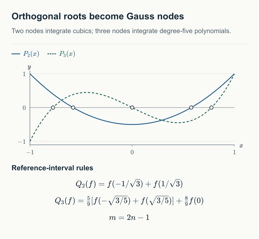
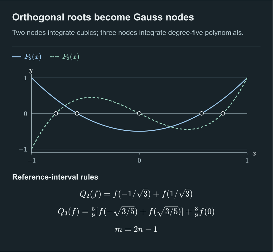
The first polynomials are
Choose the roots of as nodes. The characterization theorem and the upper bound together prove degree of precision exactly .
Weights are unique, positive and computable
Once nodes are fixed, integrating Lagrange bases gives the unique weights. Any two weight vectors exact through degree agree when applied to each , hence agree componentwise.
Positivity also has a short proof. Since has degree at most , Gaussian exactness gives
Exactness on constants gives . Reflection symmetry and uniqueness give equal weights at symmetric nodes.
| Nodes and corresponding weights | Degree of precision | |
|---|---|---|
| 1 | Node , weight | 1 |
| 2 | Nodes , weights | 3 |
| 3 | Node , weight ; nodes , each weight | 5 |
The constant and quadratic moment conditions derive these weights. For three nodes, let the outer weights be and the central weight . Then and , giving the listed values.
For four nodes the recurrence gives .
Its inner and outer pairs have the following nodes and weights:
Solve the quadratic in for the nodes, then substitute into the general weight formula proved below. The larger weights belong to the inner nodes.
Hermite interpolation proves the error
For , there is such that
Construct matching the function and derivative at every node. Existence and uniqueness follow from finite-dimensional linear algebra: homogeneous conditions force a polynomial of degree at most to be divisible by , hence zero; the data map between two dimension- spaces is invertible.
Gauss is exact on and its node values equal those of , so . At any non-node , form
The double node zeros and the additional zero give zeros. Repeated Rolle’s theorem gives . At nodes the error is zero.
Bound the continuous derivative between its minimum and maximum, multiply by nonnegative , and integrate. Divide by and apply the intermediate value theorem to obtain one common . No continuity of is needed. Finally, , so
Substitute to conclude.
The derivative coefficients are for two nodes and for three. The required derivative order increases with ; increasing the node count does not imply a fixed convergence power without checking regularity.
Interval mapping and experiment
Map the reference interval onto by
Change of variables gives
The lecture note uses for the reference variable; are auxiliary constants defined here. Write the mapped nodes and weights as and , distinguished from reference nodes and weights . The error constant gains factor : from the derivative and from the integral.
This interactive figure needs JavaScript.
The experiment lists nodes and weights already mapped to . Compare two and three nodes, then increase . Node sets are generally not nested, unlike the meshes used by Romberg. For square roots and narrow peaks, inspect the actual error alongside the node count.
Composite Gauss quadrature
Section 5.9 also applies the -point rule panel by panel. Keep as the number of nodes per panel and use for the panel count, with and . Let be the mapped rule and define
If and , then
Multiply the reference-interval error coefficient by for each panel. The local bound is . Summing over panels proves the bound. Thus recovers second-order composite midpoint, and gives fourth-order global accuracy.
The coefficient printed in Section 5.9 is inconsistent with its general-interval error expression. The proof above separates the reference coefficient from the scaling . Setting recovers the midpoint error as an independent check.
Why the implementation’s general weight formula works
The numerical experiment solves for Legendre roots by Newton iteration and uses
This equals the integral of the Lagrange basis, as follows.
Multiply and subtract the three-term recurrences at and , then sum over their indices. Adjacent terms telescope, giving the Christoffel–Darboux identity
In detail, multiply the index- recurrences by and respectively and subtract; adjacent terms have coefficients and , so summation leaves only the last term.
Set . The right side becomes . Divide by its limit at , namely , to get . The integral of the left side is one, since only is not orthogonal to constants. Hence
To prove the derivative identity, let . Its highest-degree term cancels, so its degree is at most . For every of degree at most , integration by parts gives
Thus is a multiple of . Evaluating at one gives multiplier , so ; the case is immediate directly. At a root, . Substitute into the weight formula.
The denominator is nonzero because roots are interior and simple. Numerical root solving still requires iteration limits and convergence checks, followed by independent polynomial moment checks of nodes and weights.
References
- [1] S. Rojas, “Lecture Notes on Computational Mathematics,” 2025. Course lecture note distributed with MTH2051; local source course-lecture-notes.pdf. ↩
- [2] M. U. School of Mathematics, “MTH2051: Introduction to Computational Mathematics: Course Lecture Notes and Study Workbooks,” 2026. Monash University course materials and study workbooks, Semester 2, 2026. ↩
- [3] R. L. Burden and J. D. Faires, Numerical Analysis, 9th ed. Brooks/Cole, Cengage Learning, 2011. ↩
Comments