Interpolation Error and Chebyshev Nodes

In Polynomial Interpolation, we established how to construct a unique polynomial $P_n \in P_n$ passing through $n+1$ distinct sample points $(x_i, y_i)$.

By definition, the interpolation error vanishes at the nodes:

$$E(x_i) = f(x_i) - P_n(x_i) = 0, \quad i = 0, 1, \dots, n.$$

Yet the fundamental challenge of scientific computation lies between the nodes. When we interpolate a physical system, the model must stay accurate across the continuous domain, rather than just at isolated sample points.

Does increasing the number of sample points guarantee that the polynomial converges to the underlying function?

Surprisingly, the answer is no. For equally spaced sample points, increasing the polynomial degree often triggers severe boundary oscillations, known as the Runge phenomenon.

This note develops the analytical foundations of interpolation error [1][1] R. L. Burden and J. D. Faires, Numerical Analysis, 9th ed. Brooks/Cole, Cengage Learning, 2011., [2][2] M. U. School of Mathematics, “MTH2051: Introduction to Computational Mathematics: Course Lecture Notes and Study Workbooks,” 2026. Monash University course materials and study workbooks, Semester 2, 2026.:

1. Rolle's Theorem Foundations: Moving from ordinary Rolle to generalised Rolle for multiple zeros;
2. The Interpolation Error Formula: Deriving Cauchy's remainder formula via generalised Rolle;
3. Decoupling Error Mechanisms: Separating function roughness $f^{(n+1)}(\xi)$ from nodal geometry $\prod (x - x_i)$;
4. The Runge Breakdown: Analyzing why equidistant nodes destabilize high-degree global polynomials;
5. Chebyshev Node Optimization: Exploiting the minimax property of Chebyshev polynomials to tame boundary oscillations.

Foundations: Rolle's theorem

The derivation of the interpolation error formula rests on repeated applications of Rolle's theorem.

TheoremOrdinary Rolle's theorem

Let $u < v$. If $g$ is continuous on $[u, v]$, differentiable on $(u, v)$, and satisfies $g(u) = g(v)$, then there exists some point $c \in (u, v)$ such that

$$g'(c) = 0.$$

Proof

By the Extreme Value Theorem, the continuous function $g$ attains its global minimum $m$ and maximum $M$ on the compact interval $[u, v]$.

Let $L = g(u) = g(v)$.

• If $M = m = L$, then $g$ is constant on $[u, v]$, so $g'(x) = 0$ for all $x \in (u, v)$.
• If $M > L$, $g$ attains its maximum at some interior point $c \in (u, v)$. By Fermat's theorem on local extrema, difference quotients from the left are non-negative and from the right are non-positive. Because $g$ is differentiable at $c$, these one-sided limits coincide, proving $g'(c) = 0$.
• If $m < L$, the identical argument applied to the interior minimum yields $g'(c) = 0$.

TheoremGeneralised Rolle's theorem

Let $g \in C^{n+1}([a, b])$ and suppose that $g$ has at least $n+2$ pairwise distinct zeros in $[a, b]$. Then there exists some point $\xi \in (a, b)$ such that

$$g^{(n+1)}(\xi) = 0.$$

Proof

We proceed by induction on $n$.

Base case ($n = 0$): A function with $2$ distinct zeros satisfies ordinary Rolle's theorem, guaranteeing a point where $g'(c) = 0$.

Inductive step: Assume the statement holds for $n - 1$. Let $g \in C^{n+1}([a, b])$ have $n+2$ distinct zeros:

$$z_0 < z_1 < \dots < z_{n+1}.$$

Applying ordinary Rolle's theorem to each adjacent pair $[z_i, z_{i+1}]$ for $i = 0, \dots, n$ produces $n+1$ distinct points $w_0 < w_1 < \dots < w_n$ satisfying

$$g'(w_i) = 0, \quad w_i \in (z_i, z_{i+1}).$$

Thus the derivative $g'$ belongs to $C^n([a, b])$ and possesses $n+1$ distinct zeros. By the induction hypothesis applied to $g'$, there exists $\xi \in (w_0, w_n) \subset (a, b)$ such that $(g')^{(n)}(\xi) = g^{(n+1)}(\xi) = 0$.

The interpolation error formula

TheoremCauchy-type interpolation error formula

Let $f \in C^{n+1}([a, b])$ and let $P_n \in P_n$ interpolate $f$ at $n+1$ distinct nodes $a \le x_0 < x_1 < \dots < x_n \le b$. For each fixed evaluation point $x \in [a, b]$, there exists some intermediate point $\xi_x \in (a, b)$ such that

$$f(x) - P_n(x) = \frac{f^{(n+1)}(\xi_x)}{(n+1)!} \prod_{i=0}^n (x - x_i).$$

Proof

If $x$ is one of the nodes $x_i$, then $f(x_i) - P_n(x_i) = 0$ and the product $\prod_{i=0}^n (x_i - x_i) = 0$, so the identity holds trivially for any choice of $\xi_x \in (a, b)$.

Now fix an arbitrary evaluation point $x \in [a, b]$ with $x \neq x_i$ for all $i$. Define the error at $x$ as $E(x) = f(x) - P_n(x)$, the nodal polynomial as

$$\omega_{n+1}(t) = \prod_{j=0}^n (t - x_j),$$

and the auxiliary function of a variable $t \in [a, b]$:

$$G(t) = f(t) - P_n(t) - \frac{E(x)}{\omega_{n+1}(x)} \omega_{n+1}(t).$$

Observe the roots of $G(t)$:

1. For every node $x_i$ ($i = 0, 1, \dots, n$):

$$G(x_i) = f(x_i) - P_n(x_i) - \frac{E(x)}{\omega_{n+1}(x)} \omega_{n+1}(x_i) = 0 - 0 = 0.$$

2. At the evaluation point $t = x$:

$$G(x) = E(x) - \frac{E(x)}{\omega_{n+1}(x)} \omega_{n+1}(x) = E(x) - E(x) = 0.$$

Because $x$ is distinct from all $x_i$, the function $G(t)$ has at least $n+2$ pairwise distinct zeros in $[a, b]$. Furthermore, $G \in C^{n+1}([a, b])$ because $f \in C^{n+1}$ and both $P_n$ and $\omega_{n+1}$ are polynomials.

By the generalised Rolle's theorem, there exists some $\xi_x \in (a, b)$ such that

$$G^{(n+1)}(\xi_x) = 0.$$

We now differentiate $G(t)$ exactly $n+1$ times with respect to $t$:

• Since $P_n$ is a polynomial of degree at most $n$, its $(n+1)$-st derivative vanishes identically: $P_n^{(n+1)}(t) \equiv 0$.
• The nodal polynomial $\omega_{n+1}(t) = t^{n+1} + \mathcal{O}(t^n)$ is monic of degree $n+1$, so its $(n+1)$-st derivative is the constant $(n+1)!$.

Evaluating $G^{(n+1)}$ at $\xi_x$:

$$G^{(n+1)}(\xi_x) = f^{(n+1)}(\xi_x) - 0 - \frac{E(x)}{\omega_{n+1}(x)} (n+1)! = 0.$$

Solving for $E(x) = f(x) - P_n(x)$ yields:

$$f(x) - P_n(x) = \frac{f^{(n+1)}(\xi_x)}{(n+1)!} \omega_{n+1}(x) = \frac{f^{(n+1)}(\xi_x)}{(n+1)!} \prod_{i=0}^n (x - x_i).$$

Decoupling the error mechanisms

The error formula reveals that the interpolation error decouples cleanly into two entirely independent mathematical factors:

$$|f(x) - P_n(x)| \le \underbrace{\frac{\max_{t \in [a,b]} |f^{(n+1)}(t)|}{(n+1)!}}_{\text{Analytical Roughness Factor}} \cdot \underbrace{\prod_{i=0}^n |x - x_i|}_{\text{Geometric Nodal Factor}}.$$

1. Analytical Roughness Factor: Depends strictly on the higher-order derivatives of $f$. It measures how rapidly the true function curves or bends.
2. Geometric Nodal Factor:

$$\omega_{n+1}(x) = \prod_{i=0}^n (x - x_i).$$

This term is completely independent of $f$. It is governed entirely by how the sample nodes $x_0, \dots, x_n$ are positioned across $[a, b]$.

This structural decomposition explains why polynomial interpolation can fail, and how to fix it: while we cannot alter the derivatives of $f$, we have complete freedom over the placement of the nodes.

The Runge phenomenon

The most natural choice for sampling data is equidistant spacing:

$$x_i = a + i \cdot \frac{b - a}{n}, \quad i = 0, 1, \dots, n.$$

In 1901, Carl Runge discovered that this seemingly natural choice can cause catastrophic divergence for smooth, well-behaved functions.

DefinitionRunge phenomenon

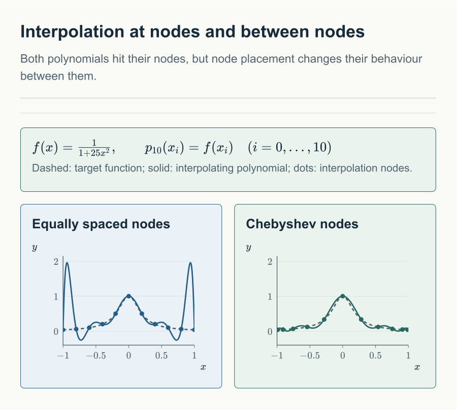
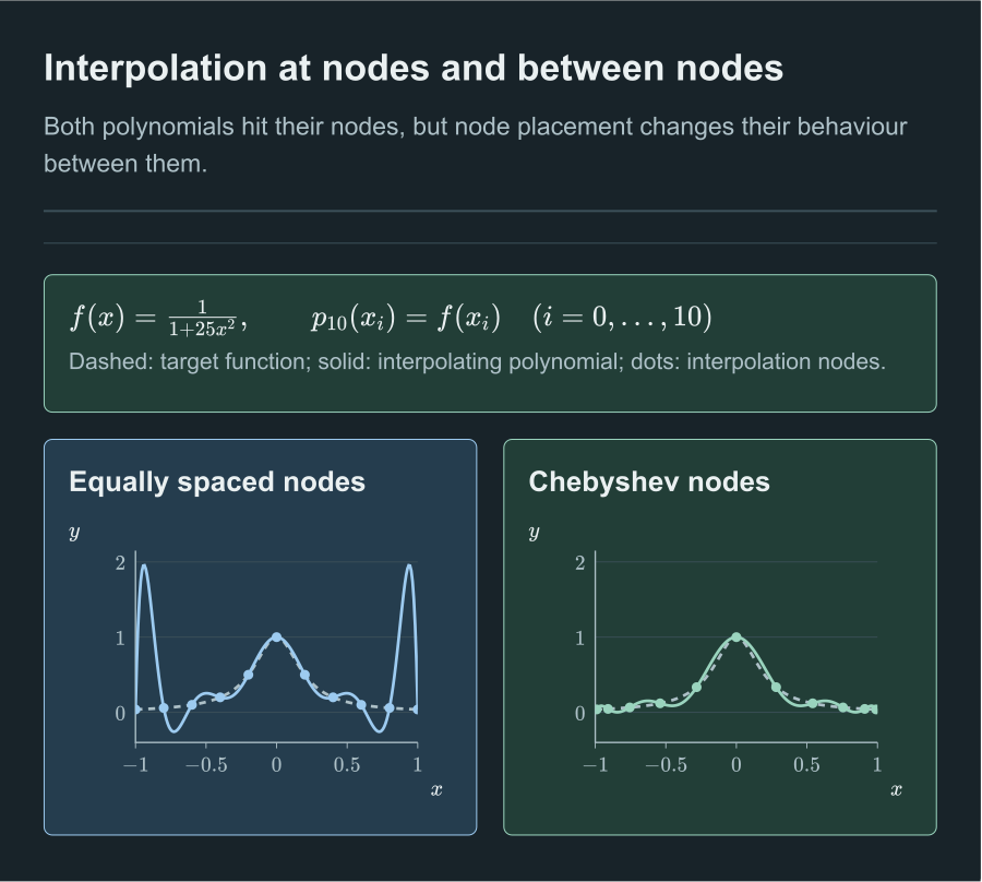
The Runge phenomenon refers to the divergence and explosive boundary oscillation that occurs when high-degree global polynomial interpolants are constructed on equally spaced nodes.

Runge's canonical counterexample is the bell-shaped function on $[-1, 1]$:

$$f(x) = \frac{1}{1 + 25x^2}.$$

Although $f$ is infinitely differentiable on the real axis, the interpolating polynomials $P_n(x)$ constructed on uniform grids do not converge to $f(x)$ as $n \to \infty$. Instead, as $n$ grows, $P_n(x)$ develops wild, growing oscillations near the boundaries $x = \pm 1$, with the maximum error growing exponentially:

$$\lim_{n \to \infty} \max_{x \in [-1, 1]} |f(x) - P_n(x)| = \infty.$$

This interactive figure needs JavaScript.

Why does this happen? The error formula provides the mathematical explanation:

• On an equidistant grid, the nodal product $\omega_{n+1}(x) = \prod_{i=0}^n (x - x_i)$ is small near the center $x \approx 0$, but surges dramatically as $x$ approaches the endpoints $\pm 1$.
• Simultaneously, although $f(x) = 1/(1+25x^2)$ is smooth on $\mathbb{R}$, in the complex plane it has poles at $z = \pm 0.2 i$. By Cauchy's integral formula, its derivatives grow at the rate $|f^{(n+1)}(\xi)| \sim (n+1)! \cdot 5^{n+1}$.
• When combined with the boundary surge of $\omega_{n+1}(x)$, the error blows up exponentially.

Chebyshev node optimization

Since the geometric factor $\omega_{n+1}(x) = \prod_{i=0}^n (x - x_i)$ governs the spatial distribution of the error, can we choose the nodes $x_0, \dots, x_n$ to minimize its maximum absolute value across the interval?

Mathematically, on $[-1, 1]$, we seek:

$$\min_{x_0, \dots, x_n \in [-1, 1]} \max_{x \in [-1, 1]} \left| \prod_{i=0}^n (x - x_i) \right|.$$

This optimal minimax problem is solved uniquely by Chebyshev nodes [1][1] R. L. Burden and J. D. Faires, Numerical Analysis, 9th ed. Brooks/Cole, Cengage Learning, 2011.:

DefinitionChebyshev polynomials

For $x \in [-1, 1]$, the Chebyshev polynomial of the first kind of degree $k$ is defined by

$$T_k(x) = \cos(k \arccos x), \quad k = 0, 1, 2, \dots$$

Using the trigonometric identity $\cos((k+1)\theta) + \cos((k-1)\theta) = 2 \cos\theta \cos(k\theta)$ with $\theta = \arccos x$, Chebyshev polynomials satisfy the three-term recurrence:

$$T_0(x) = 1, \quad T_1(x) = x, \quad T_{k+1}(x) = 2x T_k(x) - T_{k-1}(x).$$

Notice that the leading coefficient of $T_{n+1}(x)$ is $2^n$ for $n \ge 0$.

DefinitionChebyshev nodes

The Chebyshev nodes of degree $n+1$ are the $n+1$ roots of the Chebyshev polynomial $T_{n+1}(x)$ on $[-1, 1]$:

$$x_k = \cos\left( \frac{2k + 1}{2(n + 1)} \pi \right), \quad k = 0, 1, \dots, n.$$

TheoremMinimax property of Chebyshev nodes

Among all monic polynomials of degree $n+1$ on $[-1, 1]$, the scaled Chebyshev polynomial

$$\tilde{T}_{n+1}(x) = \frac{1}{2^n} T_{n+1}(x) = \prod_{k=0}^n (x - x_k)$$

uniquely minimizes the maximum absolute value on $[-1, 1]$:

$$\max_{x \in [-1, 1]} \left| \prod_{k=0}^n (x - x_k) \right| = \frac{1}{2^n}.$$

Proof

First observe that $|T_{n+1}(x)| = |\cos((n+1)\theta)| \le 1$ for all $x \in [-1, 1]$. Because the leading coefficient of $T_{n+1}$ is $2^n$, the monic polynomial $\tilde{T}_{n+1}(x) = 2^{-n} T_{n+1}(x)$ satisfies

$$\max_{x \in [-1, 1]} |\tilde{T}_{n+1}(x)| = \frac{1}{2^n}.$$

Moreover, $\tilde{T}_{n+1}(x)$ achieves its extreme values $\pm 2^{-n}$ with alternating signs at the $n+2$ Chebyshev extreme points $t_j = \cos\left(\frac{j \pi}{n+1}\right)$ ($j = 0, 1, \dots, n+1$).

Suppose there exists another monic polynomial $q \in P_{n+1}$ such that $\max_{x \in [-1, 1]} |q(x)| < 2^{-n}$. Consider the difference polynomial:

$$d(x) = \tilde{T}_{n+1}(x) - q(x).$$

Because both $\tilde{T}_{n+1}$ and $q$ are monic polynomials of degree $n+1$, their leading terms cancel, so $\deg(d) \le n$.

Now evaluate $d(x)$ at the $n+2$ points $t_j$:

• When $\tilde{T}_{n+1}(t_j) = 2^{-n}$, we have $d(t_j) = 2^{-n} - q(t_j) > 0$ because $|q(t_j)| < 2^{-n}$.
• When $\tilde{T}_{n+1}(t_j) = -2^{-n}$, we have $d(t_j) = -2^{-n} - q(t_j) < 0$.

Hence $d(x)$ alternates signs across the $n+2$ points $t_0, t_1, \dots, t_{n+1}$. By the Intermediate Value Theorem, $d(x)$ must possess at least $n+1$ distinct roots in $[-1, 1]$.

A non-zero polynomial of degree at most $n$ cannot have $n+1$ distinct roots. Therefore $d(x) \equiv 0$, establishing that no monic polynomial can achieve a smaller maximum magnitude.

Geometric intuition: the semicircle projection

Why do Chebyshev nodes resolve the Runge boundary oscillation?

Consider placing $n+1$ points uniformly on the upper half of the unit circle, with angles $\theta_k = \frac{2k+1}{2(n+1)} \pi$. Projecting these points vertically onto the horizontal diameter $[-1, 1]$ yields the Chebyshev nodes $x_k = \cos\theta_k$.

Because the circle curves down toward the horizontal axis near $\theta \approx 0$ and $\theta \approx \pi$, the projected nodes are naturally clustered more densely near the endpoints $\pm 1$ and spaced more sparsely in the interior.

This edge clustering places extra constraints precisely where the nodal product $\omega_{n+1}(x)$ previously surged, pinning down the polynomial and suppressing boundary oscillations.

For an arbitrary interval $[a, b]$, the Chebyshev nodes are mapped by an affine transformation:

$$\tilde{x}_k = \frac{a + b}{2} + \frac{b - a}{2} \cos\left( \frac{2k + 1}{2(n + 1)} \pi \right), \quad k = 0, 1, \dots, n.$$

The frontier of interpolation

Chebyshev nodes provide the optimal global solution when we are free to select sample locations.

However, in many real-world applications, two major challenges remain:

1. Derivative data: What if our sensors measure both function values and velocities or slopes $f'(x_i)$? How do we build polynomials matching values and derivatives simultaneously? This leads to Hermite Interpolation.
2. Arbitrary fixed data and local control: What if we cannot choose where points are sampled, or what if we want local edits without perturbing the entire curve? Global polynomials are fundamentally stiff: moving a single point alters the entire function across the domain. Resolving this requires partitioning the interval into low-degree polynomial pieces, leading to Spline Interpolation.

References

1. [1] R. L. Burden and J. D. Faires, Numerical Analysis, 9th ed. Brooks/Cole, Cengage Learning, 2011. a b
2. [2] M. U. School of Mathematics, “MTH2051: Introduction to Computational Mathematics: Course Lecture Notes and Study Workbooks,” 2026. Monash University course materials and study workbooks, Semester 2, 2026. ↩