Newton's Method

If bisection is a methodical, cautious explorer and general fixed-point iteration is a versatile workhorse, Newton’s method (or the Newton-Raphson method) is the Formula 1 racer of numerical analysis.

In the previous note on fixed-point iteration, we proved that an iteration sequence $x_{n+1} = g(x_n)$ converges linearly whenever the local derivative satisfies $|g'(x^*)| < 1$. This discovery prompts a bold mathematical question: can we deliberately design an iteration map $g(x)$ whose derivative vanishes completely at the root, $g'(x^*) = 0$?

Forcing $g'(x^*) = 0$ annihilates the first-order error term in Taylor expansion. The resulting sequence does not merely shrink its error by a constant factor per step; it squares the error:

$$|e_{n+1}| \approx C |e_n|^2.$$

This is quadratic convergence: an approximation with 2 correct decimal digits jumps to 4, then 8, then 16 correct digits in just three iterations! This optimal fixed-point architecture is precisely Newton’s method.

This note develops Newton’s method across three unified viewpoints:

1. Geometric: Following the local tangent line to its $x$-intercept;
2. Taylor expansion: Truncating second-order curvature terms;
3. Contraction analysis: Verifying local contraction and quadratic error decay on simple roots.

We will analyze both its extraordinary speed near simple roots and its classic failure modes (zero derivatives, periodic cycles, inflection traps), concluding with its multidimensional generalization via the Jacobian matrix.

From the tangent line

The core intuition of differential calculus is that smooth curves look like straight lines when viewed through a microscope. Newton’s method takes this local linear lens and turns it into an algorithmic engine.

Let $f$ be differentiable and suppose that $x_n$ is the current approximation to a root. The tangent line to the graph of $f$ at $(x_n, f(x_n))$ is

$$y = f(x_n) + f'(x_n)(x - x_n).$$

The next approximation $x_{n+1}$ is the exact intersection of this tangent line with the $x$-axis. Setting $y = 0$ and solving for $x$ immediately gives

$$x_{n+1} = x_n - \frac{f(x_n)}{f'(x_n)}, \qquad f'(x_n) \neq 0.$$

The same update rule emerges from a second-order Taylor expansion about $x_n$, evaluated at an unknown exact root $x^*$:

$$0 = f(x^*) = f(x_n) + f'(x_n)(x^* - x_n) + R_n, \qquad R_n = \frac{1}{2} f''(\xi_n)(x^*-x_n)^2.$$

The remainder $R_n$ is exact: it represents the nonlinear curvature that the tangent model discards, and it is quadratic in the current error $(x^* - x_n)$. Newton’s method temporarily drops $R_n$ and chooses $x_{n+1}$ to be the exact zero of the affine model $M_n(x) := f(x_n) + f'(x_n)(x-x_n)$. If $f$ were strictly linear, $f'' = 0$, so $R_n = 0$ and a single step would reach the root perfectly.

DefinitionNewton iteration

Given an initial value $x_0$, Newton’s method generates the sequence

$$x_{n+1} = x_n - \frac{f(x_n)}{f'(x_n)}$$

whenever the required derivative value $f'(x_n)$ is non-zero.

ExampleOne Newton step for a quadratic

For $f(x) = x^2 - 2$, the Newton map is

$$g_N(x) = x - \frac{x^2-2}{2x} = \frac{1}{2}\Bigl(x + \frac{2}{x}\Bigr), \qquad x \neq 0.$$

Starting from $x_0 = 3/2$ gives $x_1 = 17/12$. This calculation demonstrates the update rule only. A convergence claim still requires hypotheses and a proof.

This interactive figure needs JavaScript.

Define the Newton map $g_N(x) = x - f(x)/f'(x)$. Then $x_{n+1} = g_N(x_n)$. At a point where $f'(x) \neq 0$,

$$g_N(x) = x \quad\Longleftrightarrow\quad f(x) = 0.$$

Roots of $f$ are fixed points of $g_N$ wherever the map is defined. The condition $f'(x) \neq 0$ is needed both for the update and for this equivalence. Algebraic equivalence does not prove that an iteration converges.

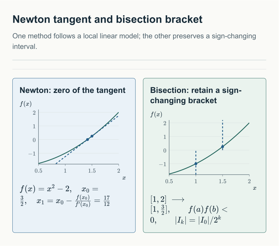
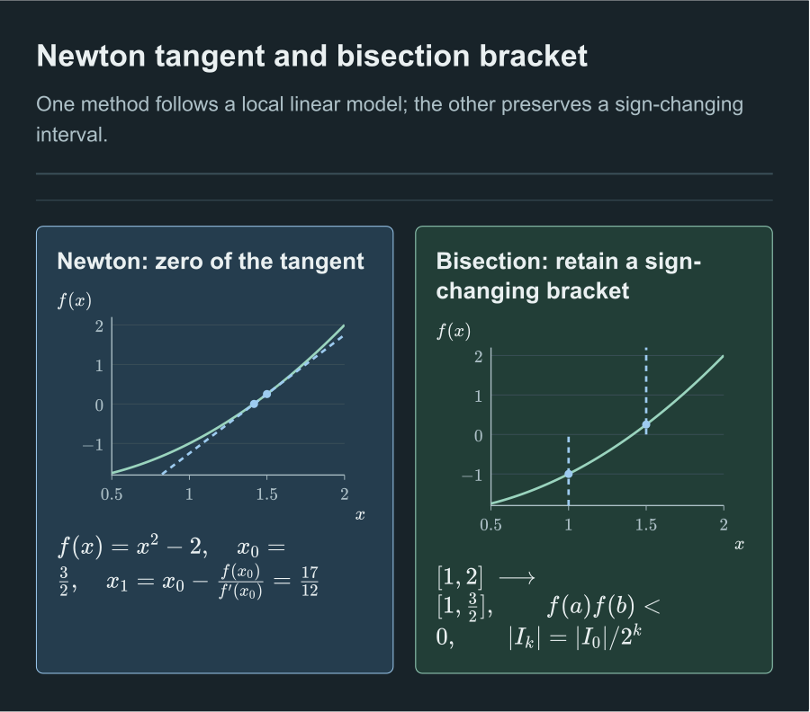
Newton follows a local tangent to its zero, while bisection retains a sign-changing bracket.

Local convergence

TheoremLocal contraction theorem

Let $g$ be continuous on the closed interval $[a,b]$, differentiable on its interior, and suppose that $g([a,b]) \subseteq [a,b]$ and there is a constant $0 \le L < 1$ such that $|g'(x)| \le L$ for every interior point. Then $g$ has a unique fixed point in $[a,b]$, and for every $x_0 \in [a,b]$ the iteration $x_{n+1} = g(x_n)$ remains in $[a,b]$ and converges to that fixed point.

A complete proof is given in the closed-interval fixed-point theorem. Its Lipschitz hypothesis follows here from the derivative bound and the mean value theorem, so all hypotheses match.

The derivative bound gives the contraction estimate through the Mean Value Theorem. The self-map keeps all iterates in the region where that estimate is available.

TheoremLocal convergence of Newton's method

Let $f \in C^2[a,b]$, and let $x^* \in (a,b)$ be a simple root, meaning $f(x^*) = 0$ and $f'(x^*) \neq 0$. Then there exists $\delta > 0$ such that, for every initial approximation $x_0 \in [x^*-\delta, x^*+\delta]$, Newton’s method generates a well-defined sequence that converges to $x^*$.

The existence of the root is an assumption: $x^*$ is given. Once the contraction and self-map conditions are established, the local contraction theorem implies that $g_N$ possesses a unique fixed point in $[x^*-\delta, x^*+\delta]$. Because $x^*$ is already a fixed point, that unique fixed point must be $x^*$. The function may possess other roots outside this local interval.

The convergence proof relies on two standard continuity lemmas.

LemmaNon-vanishing near a nonzero value

Let $h \colon [a,b] \to \mathbb{R}$ be continuous at $p \in (a,b)$. If $h(p) \neq 0$, then there exists $\delta > 0$ such that $[p-\delta, p+\delta] \subseteq [a,b]$ and $h(x) \neq 0$ for every $x$ in that interval.

Proof

Set $\varepsilon = |h(p)|/2 > 0$. Continuity at $p$ gives $\rho > 0$ such that $|x-p| < \rho$ implies $|h(x)-h(p)| < |h(p)|/2$. Because $p \in (a,b)$, the number $\delta = \tfrac{1}{2}\min(\rho, p-a, b-p)$ is positive and satisfies $[p-\delta,p+\delta] \subseteq [a,b]$ together with $\delta < \rho$. If $x$ lies in that interval, the reverse triangle inequality gives $|h(x)| \ge |h(p)| - |h(x)-h(p)| > |h(p)|/2 > 0$.

LemmaSmall values near a zero

Let $h \colon [a,b] \to \mathbb{R}$ be continuous at $p \in (a,b)$ and suppose $h(p) = 0$. Then, for every $K > 0$, there exists $\delta > 0$ such that $[p-\delta,p+\delta] \subseteq [a,b]$ and $|h(x)| \le K$ throughout that interval.

Proof

Fix $K > 0$. Continuity with $\varepsilon = K$ gives $\rho > 0$ such that $|x-p| < \rho$ implies $|h(x)| < K$. Choose $\delta = \tfrac{1}{2}\min(\rho, p-a, b-p) > 0$. Then $|x-p| \le \delta < \rho$ throughout the closed interval, so $|h(x)| \le K$.

The smaller radius $\delta < \rho$ is deliberate: continuity gives an estimate for $|x-p| < \rho$, whereas the lemmas need it on the closed interval $|x-p| \le \delta$. Apply the first lemma to $h = f'$ and the second to $h = g_N'$ with $K = L < 1$.

Proof

Step 1. Since $f \in C^2[a,b]$, the derivative $f'$ is continuous, and $f'(x^*) \neq 0$. The non-vanishing lemma applied to $h = f'$ at $p = x^*$ gives $\delta_0 > 0$ such that $I_0 = [x^*-\delta_0, x^*+\delta_0] \subseteq [a,b]$ and $f'(x) \neq 0$ on $I_0$. Hence $g := g_N$ is well-defined on $I_0$.

Step 2. On $I_0$, differentiating gives

$$g'(x) = \frac{f(x)f''(x)}{(f'(x))^2}.$$

Using $f(x^*) = 0$ gives $g'(x^*) = 0$. Fix any $L$ with $0 < L < 1$. The small-values lemma applied to $h = g'$ with $K = L$ gives a radius $\delta > 0$ such that $I = [x^*-\delta, x^*+\delta] \subseteq I_0$ and $|g'(x)| \le L$ on $I$. Thus $g$ is contractive on $I$.

Step 3. The root condition shows $g(x^*) = x^*$. Let $x \in I$. If $x = x^*$, then $g(x) \in I$. Otherwise the Mean Value Theorem gives some $\xi$ between $x$ and $x^*$, hence in $I$, and

$$|g(x) - x^*| = |g'(\xi)|\,|x-x^*| \le L\delta < \delta.$$

Therefore $g(I) \subseteq I$.

Step 4. On $I$, the map $g$ satisfies the local contraction theorem. Every Newton sequence starting in $I$ is well-defined and converges to the unique fixed point, which must be $x^*$. This is a local conclusion: the theorem asserts convergence only for sufficiently close starting values.

The logical implication is one-way: these hypotheses provide sufficient conditions for local convergence, not necessary ones. Common pitfalls include confusing sufficient conditions with necessary ones, mistaking local superlinear behavior $g'(x^*) = 0$ for a global contraction across the entire domain, and attempting to evaluate the update where $f'(x_n) \approx 0$.

Order of convergence

DefinitionOrder of convergence

Let $x_k \to x^*$. The sequence converges with order at least $p \ge 1$ if there are constants $c > 0$ and $k_0$ such that

$$|x^* - x_{k+1}| \le c |x^* - x_k|^p \qquad \text{for every } k \ge k_0.$$

When a greatest such exponent exists, it is called the order of convergence. The case $p=2$ gives at least quadratic convergence. For $p=1$, geometric or linear contraction additionally requires a bound with $c<1$; a bound with arbitrary $c>0$ alone also permits sublinear convergence.

This one-sided bound establishes an order of at least $p$, without necessarily computing the exact asymptotic limit. A higher exponent $p$ means that once iterates enter the local basin of convergence, the error vanishes with exceptional speed.

PropositionFirst-derivative classification

Let $x_{k+1} = g(x_k)$ converge to $x^*$ without reaching it in finitely many steps, and suppose $g$ is differentiable at $x^*$. Then $g(x^*) = x^*$ and

$$\frac{|x_{k+1}-x^*|}{|x_k-x^*|} \to |g'(x^*)|.$$

Therefore $0 < |g'(x^*)| < 1$ gives linear convergence, $g'(x^*) = 0$ gives superlinear convergence, and $|g'(x^*)| = 1$ is inconclusive.

Proof

Differentiability implies continuity, so taking limits in $x_{k+1} = g(x_k)$ gives $g(x^*) = x^*$. The definition of the derivative then gives the displayed ratio limit. If its value were greater than $1$, a non-terminating sequence could not converge to $x^*$.

PropositionHigher-derivative test

Let $p \ge 2$ be a positive integer, let $g \in C^p$ near $x^*$, and suppose $x_{k+1} = g(x_k) \to x^*$ with $g^{(n)}(x^*) = 0$ for $0 < n < p$. Then the iteration has order at least $p$. If $g^{(p)}(x^*) \neq 0$ and the iteration does not terminate finitely, it has exact order $p$, with asymptotic constant $|g^{(p)}(x^*)|/p!$.

Proof

Taylor’s theorem gives a point $\xi_k$ between $x_k$ and $x^*$ such that $x_{k+1}-x^* = g^{(p)}(\xi_k)(x_k-x^*)^p / p!$. Since $\xi_k \to x^*$, continuity of $g^{(p)}$ supplies both the order-at-least-$p$ bound and, when $g^{(p)}(x^*) \neq 0$, the displayed constant.

CorollaryNewton's quadratic convergence

If $f \in C^2$ near a simple root $x^*$, the Newton map satisfies $g_N'(x^*) = 0$. Hence Newton’s method has order at least $2$ in the local regime of the local convergence theorem.

Proof

A zero first derivative alone only proves superlinear convergence, so use the extra $C^2$ hypothesis directly. Taylor expansion at $x_k$ gives

$$0=f(x^*)=f(x_k)+f'(x_k)(x^*-x_k)+\tfrac12f''(\xi_k)(x^*-x_k)^2.$$

Substituting the Newton update yields

$$|x_{k+1}-x^*|=\left|\frac{f''(\xi_k)}{2f'(x_k)}\right||x_k-x^*|^2.$$

Continuity bounds the numerator and keeps the denominator away from zero locally. This supplies the uniform quadratic bound without requiring a second derivative of the Newton map.

For a root of finite multiplicity $m>1$, write $f(x)=(x-x^*)^m h(x)$ with $h(x^*)\ne0$ and $h\in C^1$ locally. Substitution into the Newton update gives

$$g_N(x)-x^*=(x-x^*)\left(1-\frac{h(x)}{mh(x)+(x-x^*)h'(x)}\right).$$

The factor tends to $1-1/m\in(0,1)$, giving local linear convergence for nonterminating iterates. This conclusion needs the stated finite-multiplicity structure; a vanishing derivative alone is not a convergence theorem.

Stopping criteria

TheoremA posteriori bound for a contraction

Let $x_{k+1} = g(x_k)$ have fixed point $x^*$, and suppose $g$ is a contraction with $0 \le \lambda < 1$ on an interval containing the relevant iterates. Then

$$|x^* - x_{k+1}| \le \frac{\lambda}{1-\lambda}\, |x_{k+1}-x_k|.$$

Proof

Let $e_k = |x^*-x_k|$. The contraction estimate gives $e_{k+1} \le \lambda e_k$. By the reverse triangle inequality, $|x_{k+1}-x_k| \ge e_k - e_{k+1} \ge (1-\lambda)e_k$. Combining this with $e_{k+1} \le \lambda e_k$ proves the bound.

When $0 < \lambda < 1$, stop only after $|x_{k+1}-x_k| < \frac{1-\lambda}{\lambda}\varepsilon$. Then the theorem guarantees $|x^*-x_{k+1}| < \varepsilon$. The rule needs a valid upper bound for $\lambda$.

TheoremStep size in the superlinear regime

Suppose $x_k \to x^*$ with order at least $p > 1$, and assume the iteration does not reach $x^*$ in finitely many steps. With $e_k = |x^*-x_k|$, let $e_{k+1} \le c e_k^p$ for all sufficiently large $k$. Then

$$\frac{e_{k+1}}{e_k} \to 0, \qquad \frac{|x_{k+1}-x_k|}{e_k} \to 1, \qquad \frac{e_{k+1}}{|x_{k+1}-x_k|} \to 0.$$

Proof

Dividing the order estimate by $e_k$ gives $0 \le e_{k+1}/e_k \le c e_k^{p-1} \to 0$. The triangle and reverse triangle inequalities give $e_k - e_{k+1} \le |x_{k+1}-x_k| \le e_k + e_{k+1}$. Dividing by $e_k$ and applying the squeeze theorem proves the middle limit, and dividing the first quotient by it proves the last.

In the superlinear regime, $|x^*-x_k| \approx |x_{k+1}-x_k|$, whereas the error of the next iterate is much smaller than the last step. The practical test $|x_{k+1}-x_k| < \varepsilon$ is therefore a conservative asymptotic proxy, not a global certificate unless extra local information is available.

Nonlinear systems

DefinitionJacobian matrix

Let $\vec{F} \colon \Omega \subset \mathbb{R}^n \to \mathbb{R}^n$ be differentiable on the open set $\Omega$, with state $\vec{x} = (x_1,\dots,x_n)^T$ and residual $\vec{F}(\vec{x}) = (F_1(\vec{x}),\dots,F_n(\vec{x}))^T$. Its Jacobian matrix $D\vec{F}(\vec{x})$ is the $n \times n$ matrix of first-order partial derivatives, with $(i,j)$ entry $\partial F_i / \partial x_j$.

PropositionNewton iteration for nonlinear systems

Let $\vec{\alpha} \in \Omega$ be an exact root, $\vec{F}(\vec{\alpha}) = \vec{0}$. Let $\vec{x}_k \in \Omega$ be the current approximation and suppose $D\vec{F}(\vec{x}_k)$ is nonsingular. The next Newton iterate is obtained by solving

$$D\vec{F}(\vec{x}_k)\, \vec{s}_k = -\vec{F}(\vec{x}_k), \qquad \vec{x}_{k+1} = \vec{x}_k + \vec{s}_k.$$

Equivalently, $\vec{x}_{k+1} = \vec{x}_k - [D\vec{F}(\vec{x}_k)]^{-1}\vec{F}(\vec{x}_k)$, although one should solve the linear system rather than invert the Jacobian.

Proof

Component-wise Taylor expansion about $\vec{x}_k$, evaluated at the root, stacks into

$$\vec{0} = \vec{F}(\vec{x}_k) + D\vec{F}(\vec{x}_k)(\vec{\alpha}-\vec{x}_k) + \vec{r}_k,$$

with a remainder $o(\|\vec{\alpha}-\vec{x}_k\|)$ from differentiability. A locally Lipschitz Jacobian, for example under $C^2$ regularity, strengthens this to a quadratic remainder. Dropping the remainder defines the affine model $\vec{M}_k(\vec{x}) := \vec{F}(\vec{x}_k) + D\vec{F}(\vec{x}_k)(\vec{x}-\vec{x}_k)$. The next iterate is the exact root of this model, which rearranges into the displayed linear system.

TheoremLocal quadratic convergence for systems

Let $\vec{F} \in C^2$ near a root $\vec{\alpha}$, and suppose $D\vec{F}(\vec{\alpha})$ is nonsingular. Then there is a neighbourhood of $\vec{\alpha}$ such that every sufficiently close $\vec{x}_0$ produces well-defined Newton iterates satisfying $\|\vec{\alpha}-\vec{x}_{k+1}\| \le c \|\vec{\alpha}-\vec{x}_k\|^2$ for a constant $c > 0$.

Proof

Put $\vec{e}_k = \vec{x}_k - \vec{\alpha}$. Taylor’s theorem gives $\vec{0} = \vec{F}(\vec{x}_k) - D\vec{F}(\vec{x}_k)\vec{e}_k + \vec{r}_k$ with $\|\vec{r}_k\| \le M \|\vec{e}_k\|^2$ locally. Nearby Jacobians remain nonsingular with uniformly bounded inverses, say of norm at most $B$. Substituting the Newton step yields $\vec{e}_{k+1} = [D\vec{F}(\vec{x}_k)]^{-1}\vec{r}_k$, hence $\|\vec{e}_{k+1}\| \le BM \|\vec{e}_k\|^2$.

To justify the uniform inverse bound, put $J_*=DF(\alpha)$. Shrink the ball so that $H=J_*^{-1}(DF(x)-J_*)$ has norm at most $1/2$. The convergent geometric matrix series $\sum_{j\ge0}(-H)^j$ is the inverse of $I+H$: multiply finite partial sums and let their residual power tend to zero. Hence $\|DF(x)^{-1}\|\le2\|J_*^{-1}\|$ throughout the ball. Choose its radius $\delta$ still smaller so that $BM\delta\le1/2$. Then the quadratic bound keeps every iterate in the ball and halves the error at least, proving existence of the entire sequence and convergence. The remainder estimate follows by integrating the locally Lipschitz Jacobian along the line segment to the root.

A standard four-step workflow for multidimensional Newton systems:

1. Formulate the residual system $\vec{F}(\vec{x}) = \vec{0}$.
2. Compute the Jacobian $D\vec{F}(\vec{x})$ and check non-singularity ($\det D\vec{F} \neq 0$).
3. Solve the linear system $D\vec{F}(\vec{x}_k)\vec{s}_k = -\vec{F}(\vec{x}_k)$ for the update step $\vec{s}_k$.
4. Update $\vec{x}_{k+1} = \vec{x}_k + \vec{s}_k$ and evaluate convergence using both step norm $\|\vec{s}_k\|$ and residual norm $\|\vec{F}(\vec{x}_{k+1})\|$.

ExamplePlanar two-link robot arm

A planar robot arm has link lengths $L_1, L_2 > 0$ and joint angles $\theta_1, \theta_2$. Given a target $(x_d, y_d)$, find joint angles that place the end of the second link at that target. Put $r = \sqrt{x_d^2 + y_d^2}$. A target can be reached only if $|L_1-L_2| \le r \le L_1+L_2$.

Resolving the two links gives

$$\begin{aligned} x(\theta_1,\theta_2) &= L_1 \cos\theta_1 + L_2 \cos(\theta_1+\theta_2), \\ y(\theta_1,\theta_2) &= L_1 \sin\theta_1 + L_2 \sin(\theta_1+\theta_2). \end{aligned}$$

The residual is $\vec{F}(\vec{\theta}) = \vec{0}$ with

$$\begin{aligned} F_1 &= L_1 \cos\theta_1 + L_2 \cos(\theta_1+\theta_2) - x_d, \\ F_2 &= L_1 \sin\theta_1 + L_2 \sin(\theta_1+\theta_2) - y_d. \end{aligned}$$

Differentiating produces

$$D\vec{F}(\vec{\theta}) = \begin{pmatrix} -L_1\sin\theta_1 - L_2\sin(\theta_1+\theta_2) & -L_2\sin(\theta_1+\theta_2) \\ L_1\cos\theta_1 + L_2\cos(\theta_1+\theta_2) & L_2\cos(\theta_1+\theta_2) \end{pmatrix}.$$

A short expansion gives $\det D\vec{F}(\vec{\theta}) = L_1 L_2 \sin\theta_2$. The Jacobian is invertible exactly when $\sin\theta_2 \neq 0$. The singular cases include a fully straight or fully folded arm.

With $L_1 = 1$, $L_2 = 0.7$, target $(1.2, 0.5)$, and start $\vec{\theta}^{(0)} = (0.3, 0.2)^T$, each Newton step solves $D\vec{F}(\vec{\theta}^{(k)})\vec{s}_k = -\vec{F}(\vec{\theta}^{(k)})$ and updates $\vec{\theta}^{(k+1)} = \vec{\theta}^{(k)} + \vec{s}_k$.

Secant and regula falsi

Both methods use the intersection of a secant line with the $x$-axis. Secant keeps the newest two points and is an open method. Regula falsi keeps a sign-changing interval and is therefore a bracketing method. That distinction explains why secant is usually faster locally, while regula falsi is safer globally.

DefinitionSecant method

Starting from two initial guesses $x_0$ and $x_1$, replace the derivative in Newton’s method by the finite-difference slope through the two most recent points:

$$x_{n+1} = x_n - f(x_n)\frac{x_n - x_{n-1}}{f(x_n)-f(x_{n-1})}.$$

The method does not preserve a bracketing interval. Under the usual local hypotheses near a simple root, its order is $p = (1+\sqrt{5})/2 \approx 1.618$. After the first two function evaluations, each new step needs one new function evaluation and no derivative.

DefinitionRegula falsi (false position)

Start with an interval $[a,b]$ such that $f(a)f(b) < 0$. The secant line through the endpoints meets the $x$-axis at

$$c = b - f(b)\frac{b-a}{f(b)-f(a)}.$$

If $f(a)f(c) < 0$, replace $b$ by $c$; otherwise replace $a$ by $c$. The sign-changing bracket is preserved. The method converges at least linearly, is often faster than bisection at first, and may stagnate when one endpoint remains fixed for many iterations.

The next note turns from solving $f(x) = 0$ to matching sampled data with a polynomial: polynomial interpolation. This page belongs to the Computational Mathematics reading path.