In pure mathematics, solutions live in the serene continuum of real numbers . We manipulate infinite Taylor series, take limits as step sizes , and write down exact roots with complete confidence. But the moment we ask physical hardware to calculate, we step into a world of unavoidable physical constraints: numbers must fit into finite bit registers (typically 32 or 64 bits), infinite processes must terminate in finite steps, and continuous functions must be represented on discrete grids.
This note establishes the foundational vocabulary and mental models for computational mathematics. Across subsequent topics, root finding, polynomial interpolation, and numerical calculus, we will repeatedly evaluate algorithms through four essential virtues:
- Accuracy: How close is the computed approximation to mathematical truth?
- Efficiency: What is the computational cost (work, memory, iterations) required to reach a target tolerance?
- Stability: Does the algorithm prevent small representation perturbations from exploding into catastrophic errors?
- Robustness: Does the algorithm behave predictably across diverse inputs and fail gracefully when assumptions break down?
From phenomena to computation
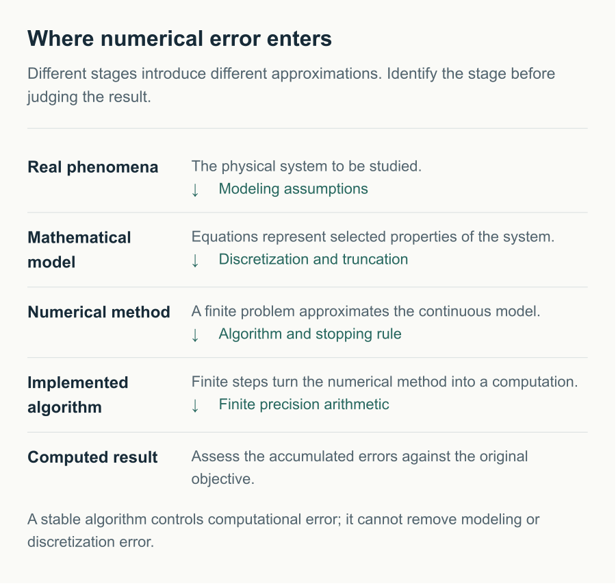
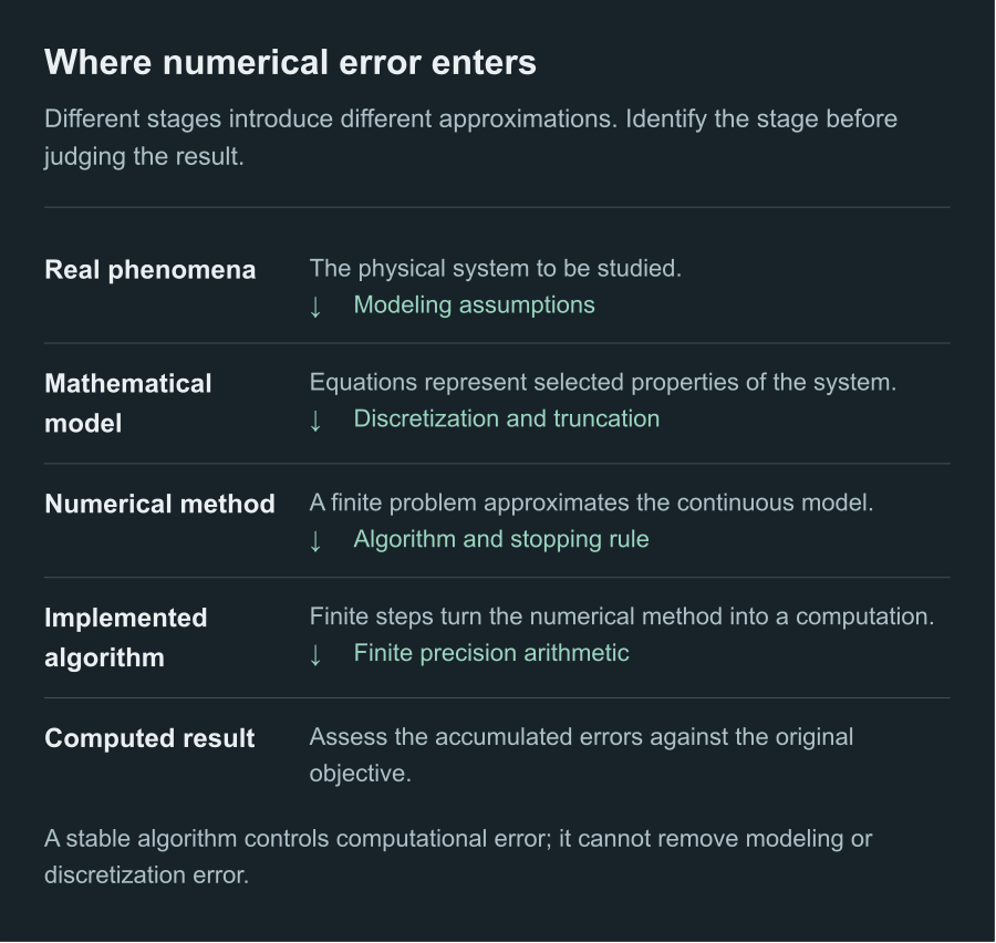
Before writing an algorithm or writing code, we must understand the transformation that carries an observed physical phenomenon into machine memory. This pipeline spans four distinct layers: the physical phenomenon, the mathematical model, the mathematical problem, and the digital computation.
A mathematical model is a deliberately simplified mathematical representation of a phenomenon. It specifies variables, parameters, assumptions, and relations among them so that questions about the phenomenon can be translated into mathematical problems.
A conservation principle might produce a partial differential equation; a balance of forces might yield a system of nonlinear algebraic equations. The modelling step decides what physics to retain and what to neglect. Crucially, solving these equations with infinite precision does not eliminate modelling error: an analytical solution to an incomplete model remains an incomplete description of reality.
A result computed to twelve decimal digits is not automatically meaningful. If an omitted physical effect (such as friction or thermal expansion) alters the true behavior by five percent, reducing numerical error from to does not improve real-world predictive validity.
A mathematical problem specifies admissible input data, the mathematical conditions that a solution must satisfy, and the desired output. Abstractly, we may write the exact solution operator as
where is the input and is the exact output.
Concrete mathematical problems include finding a root , integrating a differential equation, or solving a linear system . A problem statement is incomplete without its domain and underlying hypotheses: existence, uniqueness, differentiability, and nonzero denominators matter just as much as the algebraic formula itself.
A computation is a finite process that transforms represented input into represented output through permitted elementary operations. It includes the representation of data, the order of operations, intermediate quantities, and a rule for termination.
This definition separates the exact continuous map from what silicon hardware can execute. While real numbers contain uncountably infinite information, a floating-point register holds only finitely many bits. A computation therefore produces an approximation rather than the idealized .
A formula describes a static mathematical relationship; a computation describes an active, ordered process. Two programs implementing the exact same mathematical formula can produce dramatically different answers because they sequence operations differently or suffer from different numerical cancellation paths.
Numerical analysis is the study and design of methods for obtaining approximate solutions to mathematical problems, together with the rigorous analysis of their error, cost, sensitivity, and reliability.
The discipline asks far more than “what number did the computer output?” It investigates whether the approximation converges to the true solution, how fast the error decays, how much work is required, how representation errors propagate, and where the method can break down.
Method, algorithm, and implementation
To reason clearly about software failures and numerical bugs, we distinguish between three layers of realization: the abstract method, the executable algorithm, and the machine implementation.
A numerical method is a mathematically specified approximation strategy. It replaces an exact continuous problem by finite operations, or by a sequence of simpler problems whose solutions approach the exact solution.
A method can be based on iteration, discretisation, interpolation, linearisation, or recurrence. Its mathematical formulation identifies both the tuning parameter (such as step size , polynomial degree , or iteration count ) and the theoretical sense in which the error is expected to shrink.
A numerical algorithm is a finite, unambiguous, and executable sequence of instructions that implements a numerical method for represented data. It specifies input formats, initialisation, update rules, stopping conditions, output, and detectable failure diagnostics.
A single numerical method often admits multiple competing algorithms. For instance, evaluating an -th degree polynomial can be done by computing powers individually or via Horner’s nested multiplication. While mathematically equivalent in infinite precision, their computational complexities and roundoff propagation profiles differ substantially.
def numerical_algorithm(data, tolerance, max_steps): state = initialise(data) for step in range(max_steps): new_state = update(state, data) if error_indicator(new_state, state) <= tolerance: return new_state state = new_state raise RuntimeError("requested reliability was not established")Two foundational principles are illustrated here: stopping criteria are an integral part of an algorithm rather than an afterthought, and hitting max_steps is not a numerical answer. It is proof that the requested accuracy was not certified.
| Layer | Question | Typical source of failure |
|---|---|---|
| Problem | What exact output is required? | Ill-conditioning or non-uniqueness |
| Method | What approximation principle is used? | Truncation or discretisation error |
| Algorithm | How is the method executed finitely? | Instability or premature termination |
| Implementation | How is it realised on a machine? | Round-off, overflow, or precision loss |
“The algorithm works” is too vague a claim. A theorem about an exact method does not guarantee that its floating-point implementation will succeed, and an error-free execution run does not prove that the underlying problem is well-conditioned.
A reliable numerical algorithm must satisfy four core criteria:
- Accuracy: Its computed output is provably close to the true mathematical solution;
- Efficiency: It reaches the target tolerance with minimal computational work and memory;
- Stability: It dampens rather than magnifies intermediate round-off and representation errors;
- Robustness: It performs predictably across its declared domain and signals when its mathematical assumptions are violated.
These four properties interact constantly. A fast algorithm that frequently diverges is useless; an accurate algorithm that takes exponential time is impractical; and a stable algorithm applied to an ill-conditioned problem will still produce large forward errors because the problem itself is hyper-sensitive.
Accuracy: what “close” means
Every numerical result can inherit error from the model, the approximation, the machine arithmetic, and earlier computational steps. Reducing one source does not automatically reduce the others.
| Source | What causes it? | Concrete example |
|---|---|---|
| Modelling error | The mathematical model omits, simplifies, or misrepresents part of the physical system. | A model may not adequately describe a virus, an electric field, or the behaviour of light. |
| Truncation error | An infinite or continuous process is replaced by a finite calculation. | Stop Newton’s method after steps, retain finitely many Taylor terms, or approximate an integral with quadrature nodes. |
| Round-off error | Real numbers and arithmetic operations are represented with finite floating-point precision. | Limited significant digits, cancellation of nearby values, and overflow outside the representable range. |
| Propagation error | An earlier error is carried into later steps and may be amplified. | The forward recurrence for multiplies the initial error by increasing factors. |
Truncation extends beyond Taylor series to any method with a finite budget: a fixed number of Newton iterations, a quadrature rule with nodes, or a mesh of spacing . The Taylor remainder below is one exact description of truncation error. Its order tells how the discarded part changes as or is refined.
Computers store only finitely many significant digits, so each represented number and arithmetic result can be rounded. Two practical failure modes deserve particular attention: catastrophic cancellation, when nearly equal numbers are subtracted and reliable digits are lost, and overflow, when an intermediate magnitude lies outside the available floating-point range. The stable quadratic formula later in this note illustrates how to avoid catastrophic cancellation.
This interactive figure needs JavaScript.
Define
Integration by parts gives the forward recurrence . Let be the value produced by the same recurrence and define its error by . Then
Hence : a tiny initial round-off error is multiplied at every forward step. This is propagation error, and it explains why the recurrence is numerically unstable in that direction.
Let be the true (exact) scalar value and let be its computed approximation. The absolute error is
If , the relative error is
Absolute error has the same units as the quantity. Relative error is dimensionless and reports error compared with the scale of the answer. Neither is universally superior: relative error is undefined at and can be misleading when zero is a meaningful reference point.
| Kind | What it measures |
|---|---|
| Forward error | Distance between computed and exact result: $ |
| Backward error | Smallest perturbation of the input for which is an exact output. |
| Local error | Error introduced in one step, assuming the step starts from exact data. |
| Global error | Accumulated error after all steps over the interval or iteration history. |
| A priori bound | A guarantee derived before the computation from assumptions and parameters. |
| A posteriori estimate | An estimate derived from the computed result, residual, or refinement comparison. |
The residual is often computable even when the exact error is not. For a linear system, measures how well the computed vector satisfies the equations. A small residual implies a small forward error only when the problem is not too sensitive.
Taylor series and order
Suppose has continuous derivatives on an interval containing and . Then there is a point between and such that
where the degree- Taylor polynomial centred at is
and the remainder (truncation error) is
For the remainder is zero. Otherwise fix and set . The auxiliary function
vanishes at both endpoints , and for . Rolle’s theorem gives a zero of between the endpoints. Apply Rolle again between this zero and , where also vanishes. Repeating times gives an interior point with . Since , this says , which is the stated remainder. Rolle’s theorem is proved in interpolation error and Chebyshev nodes.
The notation makes the source of the approximation explicit: is the quantity we compute, while is what was discarded. The displacement from the expansion point is . When only its size matters, write . If stays bounded near , then . The first omitted power of determines the local order of the approximation.
Here is the signed increment from the expansion point: . Since in this example, evaluating at means approximating near . Expanding to degree one gives
where lies between and . Restrict to . Then . Since the exponential is increasing,
Multiplying by the non-negative factor gives
If , then , and hence . For , lies between and , so and . The upper bound therefore holds from both sides of zero: take and . The approximation has error as .
A family of approximations is consistent if its local approximation error tends to zero as the approximation is refined.
A method is convergent if its computed approximation tends to the exact solution in the stated limit, such as , , or .
If an error satisfies as , the approximation has order at least . Informally, once the asymptotic regime has been reached, halving reduces the leading error by approximately a factor of .
On logarithmic axes, an error law appears as a line with slope . A straight line in a log-log plot supports an asymptotic error model only over the tested range. Coarse discretisation may not yet be asymptotic, while excessive refinement may expose round-off or modelling errors.
Reporting digits without an error scale is incomplete. A more meaningful result is “ with estimated relative error below ,” together with the assumptions behind that estimate.
Efficiency: the cost of obtaining accuracy
The efficiency of a numerical algorithm describes the resources required to achieve a specified task or accuracy. Relevant resources include arithmetic operations, function evaluations, memory, communication, and elapsed time.
If evaluating requires a large simulation, the number of function evaluations may matter more than the number of scalar additions. On modern hardware, memory traffic and parallel communication can dominate arithmetic cost.
Useful distinctions include operation complexity, storage complexity, per-step cost versus the number of required updates, convergence rate, work-precision efficiency (total work to reach a target error), and scalability.
Suppose a one-dimensional discretisation uses degrees of freedom, costs work, and has error . To achieve , we need roughly
This is a work-precision law. Increasing the order can reduce the cost of high accuracy dramatically, provided the higher-order method has reasonable constants and its smoothness assumptions are satisfied.
Consider . Computing every power independently can require multiplications. Horner’s nested form
uses multiplications and additions, hence work. The method’s mathematical output is unchanged. The algorithmic organisation is better.
def horner(coefficients, x): value = 0.0 for coefficient in reversed(coefficients): value = coefficient + x * value return valueEfficiency is best understood as the computational cost required to achieve a target level of confidence, rather than raw wall-clock time alone. A fast calculation that frequently fails, requires repeated retries, or cannot certify its error bounds is rarely economical in practice.
Big-O as a shared language
We write as if there exist constants and such that whenever . For , the corresponding definition requires the bound for every beyond some threshold. The limiting regime is part of the statement.
Big-O is an eventual upper bound up to a constant. It is not an equation for an exact value, and it does not say that two functions have the same leading constant. The statement can remain true when is a loose upper bound.
For a tighter classification, means both an asymptotic upper and lower bound. The notation means , so is asymptotically smaller than .
| Use | Limit | Typical statement |
|---|---|---|
| Algorithmic cost | operations. | |
| Discretisation error | . | |
| Iteration error | . |
The grammar is shared, but the interpretation changes. In cost analysis, smaller growth is desirable. In an error law with , larger is usually desirable because the error decays faster.
If and as , then
The lower power normally dominates a sum near zero. For example, . Cancellation can improve the order, but it must be shown. It cannot be assumed from the two separate bounds.
The symbol denotes a class of bounded remainders, not one unknown scalar. From we may infer , but we cannot simply erase the two remainder terms as though they were identical.
The formal order of an iteration is a preview for later root-finding methods, not a Week 1 requirement. Let . If
for , the iteration has order . For , convergence is linear when . The case is quadratic convergence. This definition differs from the discretisation statement , even though both use the word “order.”
Big-O deliberately hides constants and the point at which asymptotic behaviour begins. A method with cost can be slower than one with cost over the entire practical range. Likewise, an method with a large error constant may initially be less accurate than an method.
Stability: controlling perturbations
Conditioning describes how sensitive the exact solution of a mathematical problem is to small perturbations in its input. A problem is ill-conditioned when small relative input changes can produce large relative output changes.
For a scalar map , a local relative condition number is when the expression is defined. Roughly,
The condition number describes the problem before an algorithm is chosen. No algorithm can recover information that the represented input does not contain.
An algorithm is stable if the perturbations introduced during its execution do not grow substantially beyond what is unavoidable from the conditioning of the problem.
The phrase “does not amplify error” is useful intuition, but it needs a reference scale. Even a stable algorithm can exhibit a large forward error on an ill-conditioned problem, because the exact problem itself amplifies input uncertainty.
Forward stability directly bounds the difference between computed and exact output. Backward stability interprets the computed output as the exact solution of a nearby problem. Mixed analysis combines input and output perturbation bounds when a purely forward or backward statement is inconvenient. Backward stability is often powerful because it separates responsibilities: the algorithm introduces only a small input perturbation, and the condition number predicts how that perturbation affects the output.
For , the textbook formula
can subtract nearly equal numbers when and is small compared with . The small root may lose most of its significant digits. A stable strategy computes the large root without cancellation and obtains the other from :
from math import copysign, sqrt
def stable_quadratic_roots(a, b, c):    discriminant = b * b - 4 * a * c    q = -0.5 * (b + copysign(sqrt(discriminant), b))    return q / a, c / q
The mathematical formula has not changed. The route through intermediate values has. This is the practical use of stability analysis: identify where information is lost, and reorganise the computation so that the machine solves a nearby problem accurately.
If one step transforms an error approximately as , repeated steps multiply the amplification factors. Stability therefore concerns a process, not only an isolated arithmetic operation. The unstable recurrence above is one instance of this mechanism.
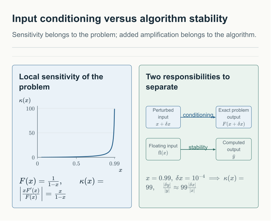
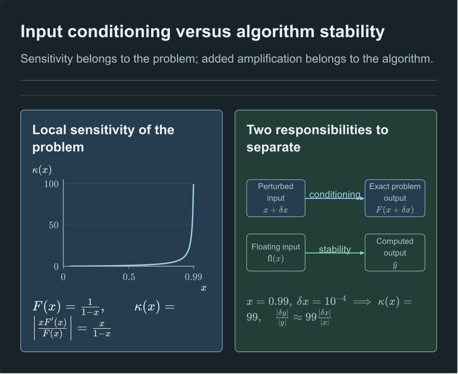
Conditioning describes sensitivity of the problem itself; numerical stability describes additional error introduced by its algorithm.
Robustness: reliable behaviour across cases
A numerical algorithm is robust over a stated domain if it produces a reliable result for a broad range of admissible inputs and behaves predictably, preferably with a diagnostic, when its assumptions or resources are insufficient.
Robustness is wider than stability. A stable update formula may still fail because an initial guess lies outside its basin of attraction, a derivative vanishes, a stopping test is misleading, or an intermediate value leaves the representable range.
Useful dimensions include domain checks, dependence on the starting guess, mixed-magnitude data, behaviour near difficult parameter regimes, termination tests that distinguish success from stagnation, and whether the method remains meaningful under available arithmetic.
A robust algorithm may combine methods. For root finding, a bracketed method offers dependable interval reduction, while a derivative-based step can be much faster near the root. A hybrid can accept the fast step when it stays inside the bracket and fall back to bisection otherwise. The safeguard adds work per step but improves the range of inputs for which the procedure can be trusted.
Useful safeguards include checking domains and finite values before an update, scaling variables to comparable magnitudes, combining absolute and relative stopping tolerances, monitoring residual reduction as well as step size, imposing iteration limits with explicit failure states, and switching methods when progress stalls.
An iteration may stagnate because floating-point numbers can no longer represent a distinct update. A stopping rule based only on may then report convergence even when the residual remains large.
A case study connecting all four properties
The derivation of finite difference formulas begins with Taylor’s theorem:
where lies between and . Rearranging gives
Thus the forward difference is first-order accurate. If is smooth, the centred difference
has truncation error . It is tempting to make as small as possible. In floating-point arithmetic, however, the numerator subtracts nearby function values and the division by magnifies their representation errors. A simplified total-error model is
where is the unit round-off. Refinement reduces truncation error but can increase round-off error. The total error has a useful intermediate scale.
This interactive figure needs JavaScript.
| Property | Question in this computation |
|---|---|
| Accuracy | How close is to , and over what range is the law observed? |
| Efficiency | How many function evaluations and precision bits are required for the target error? |
| Stability | How strongly do subtraction and division by amplify evaluation errors? |
| Robustness | Can the procedure choose or validate , detect stagnation, and handle badly scaled functions? |
Balancing the two leading terms suggests an optimal scale of order for this model. That conclusion is more useful than the slogan “smaller is better”: it combines truncation analysis, finite-precision stability, and the practical choice of a parameter.
A reusable framework
For a new numerical problem, keep the layers distinct:
- Specify the problem: inputs, desired output, domain, assumptions, and a meaningful scale for error.
- Assess conditioning: how uncertainty in the data can affect the exact answer.
- Choose a method: identify its approximation parameter and convergence assumptions.
- Design the algorithm: representation, updates, stopping tests, safeguards, and failure states.
- Analyse accuracy, efficiency, and stability as three separate questions.
- Test robustness on difficult scales and adversarial initialisations rather than typical inputs alone.
- Report the approximation together with residuals, error estimates, tolerances, and relevant assumptions.
| Property | Primary object | Diagnostic question |
|---|---|---|
| Accuracy | Output | Is the result close enough for its purpose? |
| Efficiency | Resources | What does the requested accuracy cost? |
| Stability | Perturbations | Did the algorithm add avoidable amplification? |
| Robustness | Operating domain | Will failure be controlled and visible? |
Numerical analysis studies the path from a mathematical problem to a trustworthy computed result. Big-O notation links several parts of that path: it describes how resource cost grows, how approximation error decays, and how iterative errors converge. Asymptotic order is only one dimension of quality. Constants, conditioning, floating-point stability, safeguards, and the intended use of the answer determine whether a method is genuinely useful.
The next note applies this language to bisection and fixed-point iteration. This page belongs to the Computational Mathematics reading path.
Comments