Richardson extrapolation and Romberg integration

When the leading error is known to scale with a power of the step, two approximations can be combined to cancel it. Richardson extrapolation performs this cancellation; Romberg repeatedly applies it to composite trapezoidal values.

Lecture note Sections 4.5–4.6 and 5.10–5.11 are the primary source. The target may be a derivative or an integral. In the course notation $R_{k,j}$, row $k$ counts mesh halvings and column $j$ counts extrapolations; both indices start at zero [1][1] S. Rojas, “Lecture Notes on Computational Mathematics,” 2025. Course lecture note distributed with MTH2051; local source course-lecture-notes.pdf., [2][2] M. U. School of Mathematics, “MTH2051: Introduction to Computational Mathematics: Course Lecture Notes and Study Workbooks,” 2026. Monash University course materials and study workbooks, Semester 2, 2026., [3][3] R. L. Burden and J. D. Faires, Numerical Analysis, 9th ed. Brooks/Cole, Cengage Learning, 2011..

Richardson cancels a known power

TheoremGeneral extrapolation

Suppose $p>0$, $q>p$, and

$$Q(h)=L+ch^p+O(h^q),$$

where $c$ is independent of $h$. Define

$$R(h)=\frac{2^pQ(h/2)-Q(h)}{2^p-1}.$$

Then $R(h)=L+O(h^q)$.

Proof

At $h/2$, the same leading error is $ch^p/2^p$. Multiplying by $2^p$ makes it match the coarse error, so subtraction cancels it. There remain $2^p-1$ copies of the target; division restores one copy. The linear combination of remainders is still $O(h^q)$.

A gain of two orders is not automatic. One-sided differences generally have consecutive powers, giving $q=p+1$. Symmetric differences and smooth trapezoidal quadrature have even-power structure, allowing $q=p+2$.

For example, symmetric Taylor expansions for $f\in C^5$ give

$$D_{\mathrm{cen}}(x;h)=f'(x)+\frac{h^2}{6}f'''(x)+O(h^4),$$

hence

$$\frac{4D_{\mathrm{cen}}(x;h/2)-D_{\mathrm{cen}}(x;h)}3=f'(x)+O(h^4).$$

By contrast, for $f\in C^3$ a forward difference has expansion $f'(x)+hf''(x)/2+O(h^2)$, so $2D_{\mathrm{fwd}}(x;h/2)-D_{\mathrm{fwd}}(x;h)$ guarantees only order two. Both statements follow directly from Taylor’s theorem: symmetric subtraction removes even terms, whereas a one-sided formula does not.

The fine-value correction form is

$$R(h)=Q(h/2)+\frac{Q(h/2)-Q(h)}{2^p-1}.$$

The second term estimates $L-Q(h/2)$. Its validity still depends on the expansion. Agreement between two approximations is not a universal error certificate.

Recursive extrapolation for derivatives

Section 4.6 writes derivative extrapolation as $R_k(h)$, distinct from the integral table’s $R_{k,j}$. Set $R_0(h)=D(h)$ and define

$$R_k(h)=\frac{2^{p+2(k-1)}R_{k-1}(h/2)-R_{k-1}(h)}{2^{p+2(k-1)}-1}.$$

PropositionRecursive order from a finite even-power expansion

For fixed $K\geq1$ and $p>0$, suppose

$$D(h)=f'(x)+\sum_{r=0}^{K-1}c_rh^{p+2r}+O(h^{p+2K}),$$

with coefficients independent of $h$. Then $R_k(h)=f'(x)+O(h^{p+2k})$ for $0\leq k\leq K$.

Proof

Step $k$ multiplies a term $h^{p+2r}$ by $(2^{p+2(k-1)}-2^{p+2r})/(2^{p+2r}(2^{p+2(k-1)}-1))$. The factor vanishes at $r=k-1$, and previously cancelled terms remain zero. Induction cancels the first $k$ terms; a fixed finite linear combination preserves the final remainder order.

For the centred first derivative, $p=2$, giving two more orders per step. This conclusion requires the stated finite even-power expansion and does not apply to arbitrary noisy data.

Why trapezoidal errors have even powers

A formal infinite series is not a general convergence theorem. A finite expansion is enough to justify any fixed Romberg column.

TheoremFinite Euler–Maclaurin expansion

Let $m\geq1$ be an integer and $f\in C^{2m+2}[a,b]$. On a uniform mesh $h=(b-a)/n$, the composite trapezoidal value satisfies

$$T(h)=I+\sum_{r=1}^{m} \frac{B_{2r}}{(2r)!} \bigl[f^{(2r-1)}(b)-f^{(2r-1)}(a)\bigr]h^{2r} +O(h^{2m+2}).$$

Here $B_{2r}$ are Bernoulli numbers, including $B_2=1/6$ and $B_4=-1/30$.

Proof

Define Bernoulli polynomials by $B_0(t)=1$ and, for $r\geq1$,

$$B_r'(t)=rB_{r-1}(t),\qquad \int_0^1 B_r(t)\,dt=0.$$

Integration and normalization determine them uniquely. The first ones are

$$B_1(t)=t-\frac12,\quad B_2(t)=t^2-t+\frac16,$$$$B_3(t)=t^3-\frac32t^2+\frac12t,\quad B_4(t)=t^4-2t^3+t^2-\frac1{30}.$$

The recurrence and zero mean imply $B_r(1)=B_r(0)$ for $r\geq2$. Uniqueness also yields $B_r(1-t)=(-1)^rB_r(t)$: differentiate the reflected polynomial and check its mean to prove this inductively. Thus odd-index endpoint values vanish for $r\geq3$. Write $B_r=B_r(0)$.

Extend the polynomials periodically along the mesh as $\widetilde B_r(x)=B_r(\{(x-a)/h\})$. Integrate by parts on each panel and sum:

$$T(h)-I=h\int_a^b\widetilde B_1(x)f'(x)\,dx.$$

On one panel, its boundary term is the average of the two endpoint values, and its integral term is the panel integral divided by $h$, which verifies this identity directly.

Continue integrating by parts panelwise using the polynomial derivative relation. For indices at least two, matching endpoint values cancel all internal boundaries; odd external boundary terms vanish. After order $2m$,

$$T(h)-I= \sum_{r=1}^{m}\frac{B_{2r}h^{2r}}{(2r)!} \bigl[f^{(2r-1)}(b)-f^{(2r-1)}(a)\bigr] -\frac{h^{2m}}{(2m)!} \int_a^b\widetilde B_{2m}(x)f^{(2m)}(x)\,dx.$$

Two further integrations by parts turn the last remainder into a boundary term and an integral term, both multiplied by $h^{2m+2}$. Periodic polynomials are bounded, and all needed derivatives are continuous on a compact interval. The remainder is therefore $O(h^{2m+2})$. No convergence of an infinite series is assumed.

In particular, for $f\in C^6$,

$$T(h)=I+\frac{h^2}{12}[f'(b)-f'(a)] -\frac{h^4}{720}[f'''(b)-f'''(a)]+O(h^6).$$

Matching endpoint derivatives can eliminate coefficients. Singular derivatives can invalidate the entire expansion.

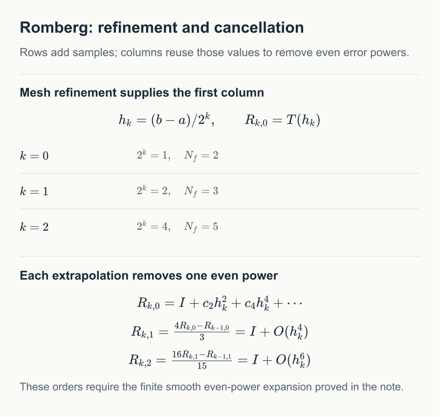
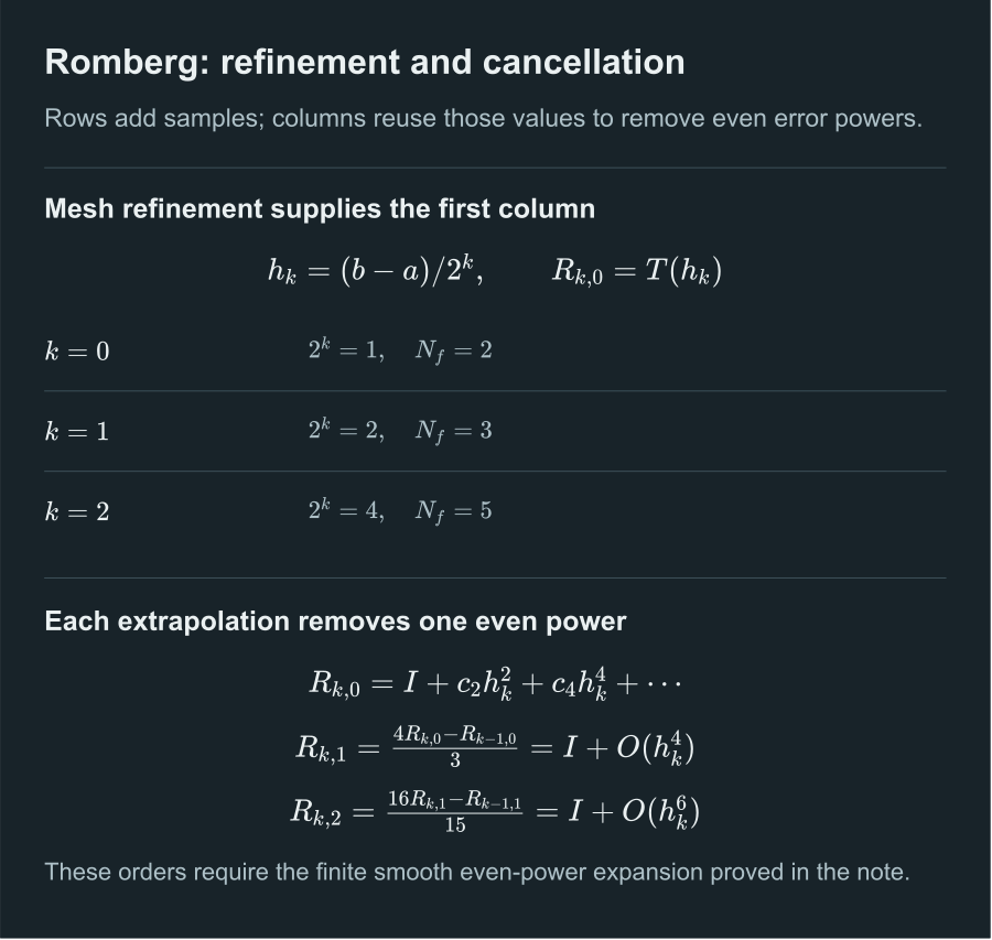
Rows sample; columns extrapolate

The lecture note allows any initial uniform mesh with spacing $h$. Here the initial mesh has one interval, so $h=b-a$. Define

$$h_k=\frac{b-a}{2^k},\qquad R_{k,0}=T(h_k),$$ $$R_{k,j}=R_{k,j-1} +\frac{R_{k,j-1}-R_{k-1,j-1}}{4^j-1}, \qquad 1\leq j\leq k.$$

TheoremAccuracy of a fixed column

For a fixed $j\geq0$, if $f\in C^{2j+2}[a,b]$, then as $k\to\infty$,

$$R_{k,j}=I+O(h_k^{2j+2}).$$

Proof

For $j=0$, use the composite trapezoidal error theorem. For $j\geq1$, take the finite expansion above with $m=j$. The first column contains even powers $h^2,\ldots,h^{2j}$ and a remainder $O(h^{2j+2})$. The preceding row has twice the current step, so a term $h^{2r}$ acquires factor $4^r$. At extrapolation step $s$, its coefficient is multiplied by

$$\frac{4^s-4^r}{4^s-1},$$

which vanishes for $r=s$. Steps $s=1,\ldots,j$ eliminate all $j$ powers. A fixed number of linear combinations preserves the remainder order. This theorem fixes the column; it does not uniformly control an ever-deeper diagonal without controlling smoothness and constants.

The first extrapolated column is exactly fine-grid Simpson quadrature by the weight identity, rather than merely another fourth-order method.

Reuse old samples

Halving the mesh preserves all old nodes and adds only midpoints. For $k\geq1$,

$$R_{k,0}=\frac12R_{k-1,0} +h_k\sum_{i=1}^{2^{k-1}}f\bigl(a+(2i-1)h_k\bigr).$$

Separate the fine trapezoidal sum into old and new nodes to prove the identity. Completing row $k$ requires $2^k+1$ total function values; further columns require no new evaluations.

Algorithm 1 Romberg table

Require: function $f$, interval $[a,b]$, maximum row $K$

1:$R_{0,0}\gets (b-a)(f(a)+f(b))/2$

2:for $k\gets1$ to $K$ do

3:$h\gets(b-a)/2^k$

4:$R_{k,0}\gets R_{k-1,0}/2+h\sum_{i=1}^{2^{k-1}}f(a+(2i-1)h)$

5:for $j\gets1$ to $k$ do

6:$R_{k,j}\gets R_{k,j-1}+(R_{k,j-1}-R_{k-1,j-1})/(4^j-1)$

7:end for

8:end for

9:return $R$

Experiment and stopping decisions

This interactive figure needs JavaScript.

For the exponential, compare the first column with the diagonal as they approach $e-1$. Switch to the square root and distinguish numerical improvement from the claimed theoretical order. Row $k$ has $2^k$ intervals; column $j$ does not add $j$ nodes.

A common stopping heuristic compares consecutive diagonal entries against a tolerance scale. Also impose a maximum row, check nonfinite values, and watch for finite-precision stagnation. Extrapolation has negative coefficients and can amplify input noise. A smaller mathematical truncation term need not improve the computed result indefinitely.

For $\int_0^1e^x\,dx=e-1$, early diagonal values are $1.859140914$, $1.718861152$, $1.718282688$, and $1.718281829$. These are reproducible examples, not unconditional guarantees. When local variation is concentrated, consider adaptive Simpson quadrature.

References

1. [1] S. Rojas, “Lecture Notes on Computational Mathematics,” 2025. Course lecture note distributed with MTH2051; local source course-lecture-notes.pdf. ↩
2. [2] M. U. School of Mathematics, “MTH2051: Introduction to Computational Mathematics: Course Lecture Notes and Study Workbooks,” 2026. Monash University course materials and study workbooks, Semester 2, 2026. ↩
3. [3] R. L. Burden and J. D. Faires, Numerical Analysis, 9th ed. Brooks/Cole, Cengage Learning, 2011. ↩