Newton–Cotes 固定等距节点,Gauss 求积则把节点位置也作为未知量。目标是:只计算 n n n
沿用 lecture note 第 5.8–5.9 节记号,在 [ − 1 , 1 ] [-1,1] [ − 1 , 1 ] x 1 , … , x n x_1,\ldots,x_n x 1 , … , x n w 1 , … , w n w_1,\ldots,w_n w 1 , … , w n
Q n ( f ) = ∑ i = 1 n w i f ( x i ) , E n ( f ) = ∫ − 1 1 f ( x ) d x − Q n ( f ) . Q_n(f)=\sum_{i=1}^n w_if(x_i),\qquad
E_n(f)=\int_{-1}^1f(x)\,dx-Q_n(f). Q n ( f ) = i = 1 ∑ n w i f ( x i ) , E n ( f ) = ∫ − 1 1 f ( x ) d x − Q n ( f ) . 这里 n n n P n P_n P n p n p_n p n [1] [1] S. Rojas, “Lecture Notes on Computational Mathematics,” 2025. Course lecture note distributed with MTH2051; local source course-lecture-notes.pdf., [2] [2] M. U. School of Mathematics, “MTH2051: Introduction to Computational Mathematics: Course Lecture Notes and Study Workbooks,” 2026. Monash University course materials and study workbooks, Semester 2, 2026., [3] [3] R. L. Burden and J. D. Faires, Numerical Analysis , 9th ed. Brooks/Cole, Cengage Learning, 2011.
代数精度的上限
定理 仅用函数值的 n 点公式的上限
任意具有 n n n 2 n 2n 2 n
证明
令 ω ( x ) = ∏ i = 1 n ( x − x i ) \omega(x)=\prod_{i=1}^n(x-x_i) ω ( x ) = ∏ i = 1 n ( x − x i ) ω 2 \omega^2 ω 2 2 n 2n 2 n
正交性怎样选出节点
使用内积
⟨ p , q ⟩ = ∫ − 1 1 p ( x ) q ( x ) d x . \langle p,q\rangle=\int_{-1}^1p(x)q(x)\,dx. ⟨ p , q ⟩ = ∫ − 1 1 p ( x ) q ( x ) d x . 定理 Gauss 精确性的充要条件
取互异节点,并令 w i = ∫ − 1 1 ℓ i ( x ) d x w_i=\int_{-1}^1\ell_i(x)\,dx w i = ∫ − 1 1 ℓ i ( x ) d x 2 n − 1 2n-1 2 n − 1 ω \omega ω n − 1 n-1 n − 1
证明
若公式精确,则对任意 deg q ≤ n − 1 \deg q\leq n-1 deg q ≤ n − 1 ω q \omega q ω q 2 n − 1 2n-1 2 n − 1
反之,对 deg p ≤ 2 n − 1 \deg p\leq2n-1 deg p ≤ 2 n − 1 p = ω q + r p=\omega q+r p = ω q + r deg q ≤ n − 1 \deg q\leq n-1 deg q ≤ n − 1 deg r ≤ n − 1 \deg r\leq n-1 deg r ≤ n − 1 ω q \omega q ω q r r r p p p
Legendre 多项式:存在性、根与递推
定义 Legendre 多项式
P n P_n P n n n n P n ( 1 ) = 1 P_n(1)=1 P n ( 1 ) = 1
定理 Rodrigues 构造与基本性质
这个多项式唯一,且
P n ( x ) = 1 2 n n ! d n d x n ( x 2 − 1 ) n . P_n(x)=\frac{1}{2^n n!}\frac{d^n}{dx^n}(x^2-1)^n. P n ( x ) = 2 n n ! 1 d x n d n ( x 2 − 1 ) n . 它有 n n n ( − 1 , 1 ) (-1,1) ( − 1 , 1 )
σ n = ( 2 n ) ! 2 n ( n ! ) 2 , ∫ − 1 1 P n ( x ) 2 d x = 2 2 n + 1 . \sigma_n=\frac{(2n)!}{2^n(n!)^2},\qquad
\int_{-1}^1P_n(x)^2\,dx=\frac2{2n+1}. σ n = 2 n ( n ! ) 2 ( 2 n )! , ∫ − 1 1 P n ( x ) 2 d x = 2 n + 1 2 . 证明
Rodrigues 式显然次数为 n n n σ n \sigma_n σ n q q q n n n ( x 2 − 1 ) n (x^2-1)^n ( x 2 − 1 ) n n − 1 n-1 n − 1 q ( n ) = 0 q^{(n)}=0 q ( n ) = 0 x = 1 x=1 x = 1 ( x − 1 ) n ( x + 1 ) n (x-1)^n(x+1)^n ( x − 1 ) n ( x + 1 ) n n n n n ! 2 n n!2^n n ! 2 n
证明根的性质:列出 ( − 1 , 1 ) (-1,1) ( − 1 , 1 ) q q q P n q P_nq P n q n n n deg q < n \deg q<n deg q < n n n n n n n P n P_n P n
平方范数同样由 Rodrigues 式分部积分 n n n
∫ − 1 1 P n 2 = σ n 2 n J n , J n = ∫ − 1 1 ( 1 − x 2 ) n d x . \int_{-1}^1P_n^2=\frac{\sigma_n}{2^n}J_n,
\qquad J_n=\int_{-1}^1(1-x^2)^n\,dx. ∫ − 1 1 P n 2 = 2 n σ n J n , J n = ∫ − 1 1 ( 1 − x 2 ) n d x . 积分 [ x ( 1 − x 2 ) n ] ′ [x(1-x^2)^n]' [ x ( 1 − x 2 ) n ] ′ ( 2 n + 1 ) J n = 2 n J n − 1 (2n+1)J_n=2nJ_{n-1} ( 2 n + 1 ) J n = 2 n J n − 1 J 0 = 2 J_0=2 J 0 = 2
J n = 2 2 n + 1 ( n ! ) 2 ( 2 n + 1 ) ! . J_n=\frac{2^{2n+1}(n!)^2}{(2n+1)!}. J n = ( 2 n + 1 )! 2 2 n + 1 ( n ! ) 2 . 代入首项系数便得范数公式。
命题 三项递推
从 P 0 = 1 P_0=1 P 0 = 1 P 1 = x P_1=x P 1 = x
( n + 1 ) P n + 1 = ( 2 n + 1 ) x P n − n P n − 1 , n ≥ 1. (n+1)P_{n+1}=(2n+1)xP_n-nP_{n-1},\qquad n\geq1. ( n + 1 ) P n + 1 = ( 2 n + 1 ) x P n − n P n − 1 , n ≥ 1. 证明
将 x P n xP_n x P n k ≤ n − 2 k\leq n-2 k ≤ n − 2 ⟨ x P n , P k ⟩ = ⟨ P n , x P k ⟩ = 0 \langle xP_n,P_k\rangle=\langle P_n,xP_k\rangle=0 ⟨ x P n , P k ⟩ = ⟨ P n , x P k ⟩ = 0 P n P_n P n ⟨ x P n , P n ⟩ = 0 \langle xP_n,P_n\rangle=0 ⟨ x P n , P n ⟩ = 0 P n + 1 P_{n+1} P n + 1 P n − 1 P_{n-1} P n − 1 ( n + 1 ) / ( 2 n + 1 ) (n+1)/(2n+1) ( n + 1 ) / ( 2 n + 1 ) x = 1 x=1 x = 1 n / ( 2 n + 1 ) n/(2n+1) n / ( 2 n + 1 )
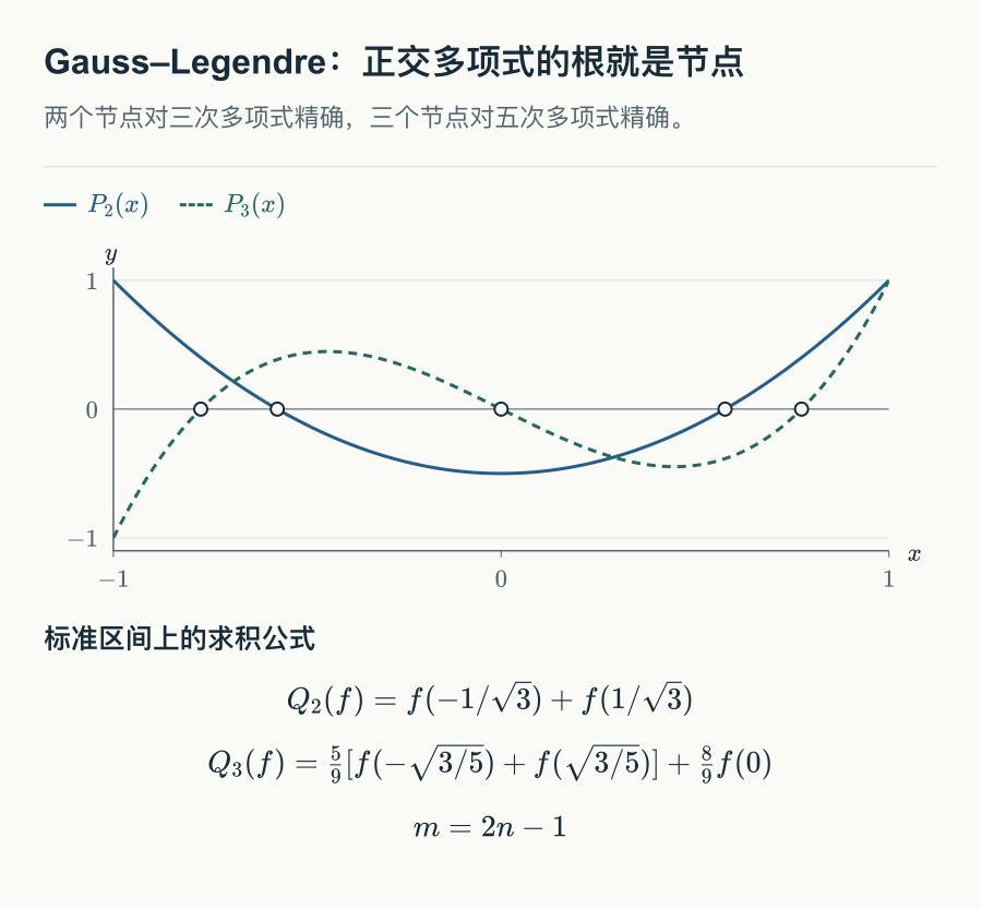
前几个多项式为
P 0 = 1 , P 1 = x , P 2 = 3 x 2 − 1 2 , P 3 = 5 x 3 − 3 x 2 . P_0=1,\quad P_1=x,\quad
P_2=\frac{3x^2-1}{2},\quad
P_3=\frac{5x^3-3x}{2}. P 0 = 1 , P 1 = x , P 2 = 2 3 x 2 − 1 , P 3 = 2 5 x 3 − 3 x . 以 P n P_n P n 恰为 2 n − 1 2n-1 2 n − 1
权重:唯一、正且可计算
节点确定后,积分 Lagrange 基给出唯一权重。唯一性来自插值:若两组权重都对次数至多 n − 1 n-1 n − 1 ℓ i \ell_i ℓ i i i i
权重为正也有简短证明。ℓ i 2 \ell_i^2 ℓ i 2 2 n − 2 2n-2 2 n − 2
w i = Q n ( ℓ i 2 ) = ∫ − 1 1 ℓ i ( x ) 2 d x > 0. w_i=Q_n(\ell_i^2)=\int_{-1}^1\ell_i(x)^2\,dx>0. w i = Q n ( ℓ i 2 ) = ∫ − 1 1 ℓ i ( x ) 2 d x > 0. 对常数精确还给出 ∑ i w i = 2 \sum_iw_i=2 ∑ i w i = 2
n n n 节点与对应权重 代数精度 1 节点 0 0 0 2 2 2 1 2 节点 ± 1 / 3 \pm1/\sqrt3 ± 1/ 3 1 1 1 3 3 节点 0 0 0 8 / 9 8/9 8/9 ± 3 / 5 \pm\sqrt{3/5} ± 3/5 5 / 9 5/9 5/9 5
这些权重可由常数和二次矩条件求出。例如三点公式设外侧权重为 u u u v v v 2 u + v = 2 2u+v=2 2 u + v = 2 2 u ( 3 / 5 ) = 2 / 3 2u(3/5)=2/3 2 u ( 3/5 ) = 2/3
四点公式由递推得到 P 4 ( x ) = ( 35 x 4 − 30 x 2 + 3 ) / 8 P_4(x)=(35x^4-30x^2+3)/8 P 4 ( x ) = ( 35 x 4 − 30 x 2 + 3 ) /8
对应节点与权重分成内外两组:
x i n n e r = ± 15 − 2 30 35 , w i n n e r = 18 + 30 36 , x_{\mathrm{inner}}=\pm\sqrt{\frac{15-2\sqrt{30}}{35}},\qquad
w_{\mathrm{inner}}=\frac{18+\sqrt{30}}{36}, x inner = ± 35 15 − 2 30 , w inner = 36 18 + 30 , x o u t e r = ± 15 + 2 30 35 , w o u t e r = 18 − 30 36 . x_{\mathrm{outer}}=\pm\sqrt{\frac{15+2\sqrt{30}}{35}},\qquad
w_{\mathrm{outer}}=\frac{18-\sqrt{30}}{36}. x outer = ± 35 15 + 2 30 , w outer = 36 18 − 30 . 节点由二次方程求得,权重可代入下文的一般权重公式验证。这也明确了较大权重应与内侧节点配对。
误差公式:Hermite 用于证明
定理 Gauss–Legendre 误差
若 f ∈ C 2 n [ − 1 , 1 ] f\in C^{2n}[-1,1] f ∈ C 2 n [ − 1 , 1 ] ξ ∈ [ − 1 , 1 ] \xi\in[-1,1] ξ ∈ [ − 1 , 1 ]
E n ( f ) = f ( 2 n ) ( ξ ) ( 2 n ) ! 2 2 n + 1 ( n ! ) 4 ( 2 n + 1 ) [ ( 2 n ) ! ] 2 . E_n(f)=\frac{f^{(2n)}(\xi)}{(2n)!}
\frac{2^{2n+1}(n!)^4}{(2n+1)[(2n)!]^2}. E n ( f ) = ( 2 n )! f ( 2 n ) ( ξ ) ( 2 n + 1 ) [( 2 n )! ] 2 2 2 n + 1 ( n ! ) 4 . 证明
构造在每个节点匹配值和导数的 Hermite 多项式 H 2 n − 1 H_{2n-1} H 2 n − 1 ω 2 \omega^2 ω 2 2 n − 1 2n-1 2 n − 1 2 n 2n 2 n
Gauss 对 H 2 n − 1 H_{2n-1} H 2 n − 1 f f f Q n ( f ) = ∫ H 2 n − 1 Q_n(f)=\int H_{2n-1} Q n ( f ) = ∫ H 2 n − 1 x x x
Φ ( t ) = f ( t ) − H 2 n − 1 ( t ) − C ω ( t ) 2 , C = f ( x ) − H 2 n − 1 ( x ) ω ( x ) 2 . \Phi(t)=f(t)-H_{2n-1}(t)-C\omega(t)^2,
\qquad C=\frac{f(x)-H_{2n-1}(x)}{\omega(x)^2}. Φ ( t ) = f ( t ) − H 2 n − 1 ( t ) − C ω ( t ) 2 , C = ω ( x ) 2 f ( x ) − H 2 n − 1 ( x ) . 每个节点是双零点,再加上 x x x 2 n + 1 2n+1 2 n + 1 C = f ( 2 n ) ( ξ x ) / ( 2 n ) ! C=f^{(2n)}(\xi_x)/(2n)! C = f ( 2 n ) ( ξ x ) / ( 2 n )!
将连续的 f ( 2 n ) f^{(2n)} f ( 2 n ) ω 2 \omega^2 ω 2 ∫ ω 2 > 0 \int\omega^2>0 ∫ ω 2 > 0 ξ \xi ξ ξ x \xi_x ξ x ω = P n / σ n \omega=P_n/\sigma_n ω = P n / σ n
∫ − 1 1 ω 2 = 1 σ n 2 2 2 n + 1 = 2 2 n + 1 ( n ! ) 4 ( 2 n + 1 ) [ ( 2 n ) ! ] 2 . \int_{-1}^1\omega^2
=\frac{1}{\sigma_n^2}\frac2{2n+1}
=\frac{2^{2n+1}(n!)^4}{(2n+1)[(2n)!]^2}. ∫ − 1 1 ω 2 = σ n 2 1 2 n + 1 2 = ( 2 n + 1 ) [( 2 n )! ] 2 2 2 n + 1 ( n ! ) 4 . 代入即得公式。
二点公式的误差系数为 1 / 135 1/135 1/135 1 / 15750 1/15750 1/15750 n n n n n n
区间变换与交互实验
将 [ − 1 , 1 ] [-1,1] [ − 1 , 1 ] [ a , b ] [a,b] [ a , b ]
x = c + d ξ , c = a + b 2 , d = b − a 2 > 0. x=c+d\xi,\qquad c=\frac{a+b}{2},\qquad d=\frac{b-a}{2}>0. x = c + d ξ , c = 2 a + b , d = 2 b − a > 0. 换元公式给出
∫ a b f ( x ) d x = d ∫ − 1 1 f ( c + d ξ ) d ξ ≈ d ∑ i w i f ( c + d x i ) . \int_a^b f(x)\,dx
=d\int_{-1}^1f(c+d\xi)\,d\xi
\approx d\sum_iw_if(c+dx_i). ∫ a b f ( x ) d x = d ∫ − 1 1 f ( c + d ξ ) d ξ ≈ d i ∑ w i f ( c + d x i ) . 讲义用 ξ \xi ξ c , d c,d c , d x ~ i = c + d x i \widetilde x_i=c+dx_i x i = c + d x i w ~ i = d w i \widetilde w_i=dw_i w i = d w i x i , w i x_i,w_i x i , w i d 2 n + 1 d^{2n+1} d 2 n + 1 2 n 2n 2 n d 2 n d^{2n} d 2 n d d d
这个交互图需要启用 JavaScript。
实验列出的节点与权重已经映射到 [ 0 , 1 ] [0,1] [ 0 , 1 ] n n n
复合 Gauss 求积
讲义第 5.9 节还把 n n n n n n N N N h = ( b − a ) / N h=(b-a)/N h = ( b − a ) / N y j = a + j h y_j=a+jh y j = a + j h Q n ( f ; [ y j , y j + 1 ] ) Q_n(f;[y_j,y_{j+1}]) Q n ( f ; [ y j , y j + 1 ])
Q n , N ( f ) = ∑ j = 0 N − 1 Q n ( f ; [ y j , y j + 1 ] ) . Q_{n,N}(f)=\sum_{j=0}^{N-1}Q_n(f;[y_j,y_{j+1}]). Q n , N ( f ) = j = 0 ∑ N − 1 Q n ( f ; [ y j , y j + 1 ]) . 命题 复合 Gauss 的全局阶数
若 f ∈ C 2 n [ a , b ] f\in C^{2n}[a,b] f ∈ C 2 n [ a , b ] ∣ f ( 2 n ) ∣ ≤ B 2 n |f^{(2n)}|\leq B_{2n} ∣ f ( 2 n ) ∣ ≤ B 2 n
∣ I − Q n , N ( f ) ∣ ≤ ( n ! ) 4 ( 2 n + 1 ) [ ( 2 n ) ! ] 3 ( b − a ) B 2 n h 2 n . |I-Q_{n,N}(f)|\leq
\frac{(n!)^4}{(2n+1)[(2n)!]^3}(b-a)B_{2n}h^{2n}. ∣ I − Q n , N ( f ) ∣ ≤ ( 2 n + 1 ) [( 2 n )! ] 3 ( n ! ) 4 ( b − a ) B 2 n h 2 n . 证明
标准区间误差先乘每块的缩放因子 ( h / 2 ) 2 n + 1 (h/2)^{2n+1} ( h /2 ) 2 n + 1 B 2 n h 2 n + 1 ( n ! ) 4 / ( ( 2 n + 1 ) [ ( 2 n ) ! ] 3 ) B_{2n}h^{2n+1}(n!)^4/((2n+1)[(2n)!]^3) B 2 n h 2 n + 1 ( n ! ) 4 / (( 2 n + 1 ) [( 2 n )! ] 3 ) N = ( b − a ) / h N=(b-a)/h N = ( b − a ) / h n = 1 n=1 n = 1 n = 2 n=2 n = 2
实验中一般权重公式的依据
数值实现用 Newton 法求 P n P_n P n
w i = 2 ( 1 − x i 2 ) [ P n ′ ( x i ) ] 2 . w_i=\frac{2}{(1-x_i^2)[P_n'(x_i)]^2}. w i = ( 1 − x i 2 ) [ P n ′ ( x i ) ] 2 2 . 下面说明这个公式与积分 Lagrange 基一致。
证明
三项递推相乘相减并逐项相加,内部项抵消,得到 Christoffel–Darboux 恒等式
∑ k = 0 n − 1 2 k + 1 2 P k ( x ) P k ( y ) = n 2 P n ( x ) P n − 1 ( y ) − P n − 1 ( x ) P n ( y ) x − y . \sum_{k=0}^{n-1}\frac{2k+1}{2}P_k(x)P_k(y)
=\frac n2\frac{P_n(x)P_{n-1}(y)-P_{n-1}(x)P_n(y)}{x-y}. k = 0 ∑ n − 1 2 2 k + 1 P k ( x ) P k ( y ) = 2 n x − y P n ( x ) P n − 1 ( y ) − P n − 1 ( x ) P n ( y ) . 其推导只需将第 k k k P k ( y ) P_k(y) P k ( y ) P k ( x ) P_k(x) P k ( x ) k + 1 k+1 k + 1 k k k y = x i y=x_i y = x i n P n − 1 ( x i ) P n ( x ) / ( 2 ( x − x i ) ) nP_{n-1}(x_i)P_n(x)/(2(x-x_i)) n P n − 1 ( x i ) P n ( x ) / ( 2 ( x − x i )) x → x i x\to x_i x → x i n P n − 1 ( x i ) P n ′ ( x i ) / 2 nP_{n-1}(x_i)P_n'(x_i)/2 n P n − 1 ( x i ) P n ′ ( x i ) /2 ℓ i ( x ) \ell_i(x) ℓ i ( x ) x x x k = 0 k=0 k = 0
w i = 2 n P n − 1 ( x i ) P n ′ ( x i ) . w_i=\frac{2}{nP_{n-1}(x_i)P_n'(x_i)}. w i = n P n − 1 ( x i ) P n ′ ( x i ) 2 . 最后证明导数恒等式。多项式 G = ( 1 − x 2 ) P n ′ + n x P n G=(1-x^2)P_n'+nxP_n G = ( 1 − x 2 ) P n ′ + n x P n n − 1 n-1 n − 1 deg q ≤ n − 2 \deg q\leq n-2 deg q ≤ n − 2
∫ − 1 1 G q = ∫ − 1 1 P n [ ( n + 2 ) x q − ( 1 − x 2 ) q ′ ] = 0. \int_{-1}^1Gq
=\int_{-1}^1P_n\bigl[(n+2)xq-(1-x^2)q'\bigr]=0. ∫ − 1 1 Gq = ∫ − 1 1 P n [ ( n + 2 ) x q − ( 1 − x 2 ) q ′ ] = 0. 因此 G G G P n − 1 P_{n-1} P n − 1 x = 1 x=1 x = 1 n n n G = n P n − 1 G=nP_{n-1} G = n P n − 1 n = 1 n=1 n = 1 ( 1 − x i 2 ) P n ′ ( x i ) = n P n − 1 ( x i ) (1-x_i^2)P_n'(x_i)=nP_{n-1}(x_i) ( 1 − x i 2 ) P n ′ ( x i ) = n P n − 1 ( x i )
这也说明分母不会为零:所有根都在开区间内,且都是单根。实际求根仍需限制迭代次数,检查收敛,并通过多项式矩验证节点和权重。
参考文献
[1] S. Rojas, “Lecture Notes on Computational Mathematics,” 2025. Course lecture note distributed with MTH2051; local source course-lecture-notes.pdf. ↩ [2] M. U. School of Mathematics, “MTH2051: Introduction to Computational Mathematics: Course Lecture Notes and Study Workbooks,” 2026. Monash University course materials and study workbooks, Semester 2, 2026. ↩ [3] R. L. Burden and J. D. Faires, Numerical Analysis , 9th ed. Brooks/Cole, Cengage Learning, 2011. ↩
评论