The Question Supervised Learning Cannot Answer
Supervised learning is, at its core, a curve-fitting problem with a teacher in the loop. You are handed a fixed dataset of input-output pairs, and for every input there is a ground-truth label telling you exactly what the correct output should have been. The learning signal, a loss between prediction and label, is available immediately, for every single example, independent of what the model predicted for any other example.
Reinforcement learning removes the teacher. There is no ground-truth label for “the correct action” in a given situation. Instead, an agent interacts with a world, takes actions, and receives a scalar reward that says how good the outcome was, not which action would have been best, not what it should have done differently, just a number. Worse, that number may not even arrive until long after the action that caused it. The learning problem shifts from “match this label” to “figure out, from consequences alone, which of your past choices were actually good ideas.”
This is not a cosmetic difference. It changes what kind of mathematical object you are even allowed to write down as your training signal.
| Dimension | Supervised learning | Reinforcement learning |
|---|---|---|
| Training signal | Ground-truth labels | Reward signals |
| Data source | Usually a fixed dataset | Agent-environment interaction |
| Data assumption | Often treated as i.i.d. | Sequential and policy-dependent |
| Feedback timing | Usually immediate label/loss | May be delayed |
| Goal | Predict labels well | Maximize expected cumulative reward |
The last row of that table is doing more work than it looks like. “Predict labels well” is a well-posed statistical estimation problem the moment you fix a dataset. “Maximize expected cumulative reward” is not yet well-posed at all: it requires defining what an agent, an environment, an action, and a return even are.
That is the honest starting position of this chapter. Reinforcement learning does not begin with an algorithm, or even with an objective function. It begins with the work of making its own goal statement mean something. The rest of this chapter assembles the four pieces that turn the slogan into a specification: the loop that generates the data, the set actions are drawn from, the dynamics that respond to them, and the two obstacles that make the whole thing hard.
The Loop Every RL Problem Runs On
With no dataset to be handed, something has to produce the data instead. That something is a specific back-and-forth between two roles, and getting the vocabulary for that exchange precise is worth doing before anything else.
The agent is the decision-making system in a reinforcement-learning problem. It can be a lookup table, a rule-based controller, a neural-network policy, a robot controller, a game-playing strategy, or any other system that chooses actions given states or observations.
The environment is the external system the agent interacts with. It receives actions, updates its internal state, and returns observations and rewards.
One interaction step proceeds as follows:
- The agent receives a state or observation.
- The agent selects an action from the action space.
- The environment receives the action.
- The environment transitions to the next state or observation.
- The environment returns a scalar reward signal.
Compactly:
Do not narrow “agent” to the current AI-agent or LLM-agent meaning. In reinforcement learning, the term predates that usage by decades: the agent is simply the source of behavior, whatever mechanism produces it.
Do not conflate the state transition with the reward. The transition describes what changed in the world; the reward is a separate, scalar judgment of how good that change, or the action that caused it, was. A system can transition states without any notion of good or bad attached; reinforcement learning requires both.
Notice what this loop quietly declines to specify. Step 2 says the agent selects an action “from the action space” without saying what that set contains. Steps 3 through 5 say the environment responds without saying what governs the response. Those two omissions are the next two sections, and neither is a technicality: the first constrains which algorithms are even applicable, and the second draws the line that the entire model-based/model-free split falls along.
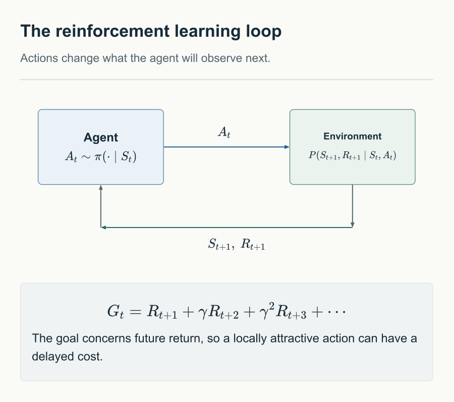
An action changes the next state and reward, so its value depends on the subsequent interaction.
Action Space
Every step of the loop routes through a choice: which action does the agent select? The set of actions it is legally allowed to choose from is the action space, and its shape, finite and enumerable, or an infinite continuum, turns out to constrain which algorithms are even applicable.
The action space, written , is the set of all legal actions the agent can choose from. When legal actions depend on the current state, write .
A discrete action space contains finitely or countably many actions:
for example .
A continuous action space is usually a subset of a real vector space:
for example with : a robot’s steering angle and speed, or a vector of joint torques.
In a small discrete action space, a value-based method can pick the best action by brute-force enumeration:
That trick stops being available the moment is a continuum: there are infinitely many candidate actions, and evaluating at every one of them is not a finite computation. This single constraint is why policy-gradient, actor-critic, and other methods that let a policy output a continuous action or a continuous action distribution, rather than search over one, are the natural fit for continuous-control problems. The action-space shape is not a footnote; it is one of the first design decisions the rest of an RL method has to be compatible with.
Both branches of this definition come back later in this series: discrete action spaces get the categorical policy, and continuous action spaces get the diagonal Gaussian policy, in Policies as Probability Distributions.
Model in Reinforcement Learning
The agent chooses actions; something else has to determine what happens as a result. That something is the environment’s dynamics, usually called the model, and it is worth being precise about the fact that it answers a completely different question than the policy does.
The transition model gives the distribution over next states given the current state and action:
The reward model gives the reward produced by a state-action pair (or state-action-next-state triple):
| Concept | Question it answers |
|---|---|
| Policy | What action should the agent take in this state? |
| Model | If the agent takes this action, how might the environment change, and what reward may result? |
The policy lives inside the agent; the model lives inside the environment. Confusing the two is a common source of bugs in both notation and code: a policy is a decision rule you control and optimize, a model is a fact about the world you can, at best, observe or approximate.
Model-based methods know or explicitly learn an approximation of the environment’s transition and reward dynamics, and use that approximation for planning or decision-making.
Model-free methods do not explicitly represent the transition dynamics. They learn a policy, a value function, or both, directly from interaction, without ever writing down an approximation of .
This split is about whether the dynamics themselves are explicitly represented somewhere in the learner. It has nothing to do with whether a neural network is involved, since both model-based and model-free methods routinely use one.
The split also has a scheduling consequence for this series. When and are known in advance, they are exactly the ingredients that make the exact backups of Planning with a Known Model computable without sampling anything. When they are not known, that entire family of methods becomes unavailable at once, and Policy Gradient estimates the same underlying quantities from rollouts instead. Which side of this line a problem falls on decides most of what follows.
Two Obstacles With No Supervised Counterpart
The loop is specified, the action set is specified, the dynamics are specified. It is tempting to conclude the hard part is now simply “pick good actions.” Two structural obstacles already make that harder than it sounds, and neither has a real counterpart in ordinary supervised learning. Both are worth naming precisely before any algorithm tries to work around them.
Delayed Reward and Credit Assignment
A reward is delayed when the usefulness of an action becomes visible only many steps later, or only once an episode ends. Credit assignment is the resulting problem of deciding which earlier actions should be credited, or blamed, for a later reward.
Consider an interaction sequence
in which the only informative reward arrives at the very last step, . A supervised learner facing a sequence like this would simply have no signal at all for of its decisions. A reinforcement-learning method has to infer, from that single terminal number, which of the actions actually contributed to the outcome, a genuinely different inferential problem than fitting a label.
The tool that eventually resolves this is return: aggregating reward over time rather than looking at one step in isolation, which Return, Value, and the Bellman Equation defines precisely. Further along, the “reward-to-go” refinement in Policy Gradient sharpens it, restricting credit for an action to the reward that arrives causally after it.
Exploration and Exploitation
Exploitation means choosing actions already believed to produce high reward. Exploration means trying actions whose consequences are still uncertain, in order to find out whether they are better.
The two pull in opposite directions, and getting the balance wrong fails in two different ways: too little exploration traps the agent in a locally good behavior it never learns to improve on; too much exploration wastes reward and destabilizes learning by never committing to what already works. A stochastic policy (one that assigns nonzero probability to more than one action, ) is one natural mechanism for exploration, since it keeps trying alternatives by construction. It is not the only one: explicit action noise, optimistic value initialization, and uncertainty-aware action selection all serve the same purpose through different means.
This is one of two genuinely distinct reasons a policy is worth making stochastic in the first place. The other is purely mathematical, and is the subject of Policies as Probability Distributions.
Where This Leaves the Goal Statement
“Maximize expected cumulative reward” is still not a well-posed problem at the end of this chapter, and it is worth being clear about exactly what is still missing rather than glossing over it. The interaction loop says how data gets generated. The action space says what may be chosen. The model says how the world responds. What none of them yet supply is a precise definition of the thing being maximized: “cumulative reward” over an unboundedly long future is not yet a convergent quantity, and “expected” is not yet an expectation over anything specified.
Closing that gap needs one structural assumption about states, which The Markov Ladder supplies, and then the return and value machinery built on top of it.
Comments