The Waste in On-Policy Sampling
Policy Gradient ended with an estimator that works:
The whole of this chapter is contained in one detail of that line: the subscript. The expectation is taken over trajectories drawn from , the distribution induced by the current parameters. Take a single gradient step, and is no longer the that generated the batch. Every sample in hand is now drawn from the wrong distribution, and the estimator that made the step has no license to make a second one.
So the loop is forced: collect a batch, take one step, discard the batch, collect again. Each trajectory funds exactly one update and is then thrown away. Nothing is recomputed and nothing is wasted twice; the waste is that expensive samples are used once.
How expensive depends on the problem, and for the domains this series is heading toward, the answer is: expensive enough that it dominates everything else. A single sample means generating a full token sequence, or running an entire denoising chain. The gradient step is cheap by comparison. Spending a whole round of generation to buy one step is the central inefficiency of on-policy policy gradient, and it is what Proximal Policy Optimization exists to fix.
The question this chapter answers is therefore narrow and practical:
Can one batch of trajectories fund many gradient steps?
The answer is yes, conditionally, and the rest of the chapter is about what the condition costs.
What We Are Estimating
Before touching the sampling machinery, it is worth being precise about the object being multiplied by the gradient, since every step below manipulates it and the final objective splits into cases according to its sign.
For a policy , the advantage function is
Both terms come from Return, Value, and the Bellman Equation: is the expected return from taking in and following afterward, and is the expected return from when the first action is also drawn from . The difference is what taking specifically buys, relative to what the policy would have done on its own.
That "relative to" is not informal. It is exactly what the following says.
For every state ,
Expand the definition and split the expectation:
The first sum is , by the state-value-from-action-value proposition of the previous chapters. The second sum is , since is a probability distribution. The two terms are therefore both and cancel.
This fixes the meaning of the sign, which is the only property of the clipped objective will actually use:
- : taking is better than what does on average from . The update should make more likely.
- : taking is worse than 's own average. The update should make less likely.
Because the mean is exactly zero, "better than average" is a statement about measuring itself. An advantage is not a score of an action in isolation; it is a comparison against the policy that is being improved, and it is recomputed every time that policy changes. That last clause is worth holding on to, because it is a second reason the samples in a batch go stale.
In practice is not known and must be estimated from the batch. Policy Gradient built the estimator this chapter inherits, with , and proved there that subtracting any action-independent baseline leaves the gradient direction unbiased. Nothing below depends on how is obtained, only on the fact that it estimates and carries a sign.
Importance Sampling
The obstacle is that the expectation is over the wrong distribution. There is a standard identity for exactly that situation.
Let and be distributions over the same space, and let be a function such that for every with . Then
Write the left side as a sum and insert , which is legitimate at every contributing a nonzero term, by the support condition:
Points where contribute zero to both sides and may be ignored regardless of . For continuous the sums become integrals and the argument is unchanged.
The condition is not decoration. Read it in the direction this chapter needs, with the old policy and the new one: any action the new policy would like to take must have had nonzero probability under the old policy. An action the old policy never proposes is invisible to the estimator, no matter how good the new policy thinks it is, because no sample of it exists to reweight. Reuse can only redistribute credit among behaviours already sampled; it cannot discover new ones. This is a real failure mode for a policy that has already collapsed onto a narrow set of actions, and it is a structural reason on-policy methods cannot be replaced by reuse indefinitely.
Applying the identity to trajectories exposes the piece of luck that makes any of this computable.
The trajectory factorization from the previous chapter gives
and the same expression with in place of . Both the initial-state term and every transition term come from the environment and carry no dependence on the policy parameters, so they appear identically in numerator and denominator and cancel factor by factor, leaving only the policy terms.
This is the same cancellation that made the policy gradient computable without a model, appearing a second time for a different reason. There it removed of terms the agent does not control; here it removes those terms from a ratio. In both cases the conclusion is that a quantity which appears to require knowing the environment's dynamics does not.
where the expectation is over timesteps of trajectories sampled with , and estimates .
The reason is worth optimizing at all is that its gradient, at the point where the samples were collected, is the object the previous chapter derived.
Differentiate the ratio and evaluate at . The denominator does not depend on , so
the last step being the log-derivative identity from the previous chapter, read right to left. Since does not depend on ,
which is exactly the policy-gradient estimator.
The proposition is easy to over-read. It does not say , and it does not say . It says the two gradients agree at one point, , and says nothing whatsoever about any other .
This distinction is the hinge of the entire chapter. is a local stand-in for , accurate to first order at the place the batch was drawn, and its licence expires as moves. Treating as the thing to be maximized, rather than as a model that is trustworthy near and meaningless far from it, is precisely the error every mechanism in the rest of this chapter exists to prevent.
Honesty requires flagging a gap between the trajectory identity and the surrogate defined above. The importance sampling lemma applied to whole trajectories produces the product as the weight on . The surrogate instead attaches a single to each timestep's advantage.
These are not the same object. Passing from one to the other additionally assumes that the distribution over states visited does not shift much between and : the per-timestep form reweights the action taken at , but not the probability of having arrived at at all. That assumption is exactly as local as the first-order guarantee above, and it fails in the same regime, when the policies drift apart. The per-timestep surrogate is thus a second approximation layered on the first, and both are paid for by the same remedy. The chapter's argument does not depend on quantifying this gap, only on noting that it points the same direction as everything else here: near is safe, far is not.
Unbiased Is Not Enough
The importance sampling identity is exact. It is tempting to conclude that reuse is therefore free, and the conclusion is wrong. The identity equates two expectations, and expectations are statements about infinitely many samples. What a finite batch delivers depends on variance.
Under the conditions of the importance sampling lemma,
which is to be compared against
Apply to under . The second term is by the lemma. For the first,
The two expressions differ in exactly one place: the reweighted estimator carries an extra factor of inside the second moment. Wherever the new policy places substantially more mass than the old one, that factor is large, and it enters the variance multiplicatively while contributing nothing to the mean.
The severity is worth stating plainly rather than as a caution about "large" variance. The extra factor is unbounded: can be arbitrarily large at points where is small but nonzero, so can diverge even when is bounded and both and are perfectly ordinary distributions. An estimator can be unbiased and have infinite variance simultaneously. Unbiasedness constrains where the estimator points on average across infinitely many draws; it says nothing about what a batch of a few thousand will hand you. In that regime a handful of samples with enormous ratios dominate the average, and the estimate is noise wearing the shape of a gradient.
That is the first failure. The second is already on the table and is more fundamental.
The proposition of the previous section holds at . As moves away, nothing has been established about the relationship between and at all. Push far enough and increasing carries no implication about : the optimizer is diligently climbing a model whose only guarantee was local, and which it has left behind. The per-timestep approximation flagged above degrades on the same schedule, for the same reason.
Two independent failures, one conclusion.
The variance of the reweighted estimator grows with the divergence between and . The validity of the surrogate as a model of is guaranteed only at and degrades as leaves it.
Reuse is legitimate, but only locally. Every remaining section of this chapter is a consequence of that sentence: first making "locally" precise, then finding a cheap way to enforce it.
How Far Is Far: KL Divergence
"Stay near " is not yet a usable instruction, because it does not say near in what sense. The naive reading, near in parameter space, is the wrong one: has no fixed relationship to how much the policy's behaviour changed. The same parameter displacement can leave a policy essentially unchanged in one region of parameter space and transform it completely in another. What the previous section's failures actually depend on is the divergence between two distributions, so that is what has to be measured.
For distributions and over the same space, with wherever ,
, with equality if and only if almost everywhere under .
Apply Jensen's inequality to the concave function :
so . Because is strictly concave, Jensen holds with equality exactly when is constant -almost everywhere; since both and sum to one, that constant must be , giving almost everywhere.
Calling a distance is an abuse worth refusing explicitly, because the habit causes real errors of intuition. It is not symmetric: in general, and the two differ in what they penalize. It does not satisfy the triangle inequality. It is a divergence: non-negative, zero exactly on the diagonal, and nothing more. When a direction is chosen below, it is chosen, not conventional.
Two facts connect this to the ratio, and they turn out to be the same fact.
For any state , with expectation over the old policy's own actions,
using the support condition to cancel, and that is a distribution.
Directly from the definitions:
Combining the two propositions, and using that is convex:
The corollary is worth pausing on, because it says the divergence being controlled and the ratio being clipped are not two topics. The ratio averages to exactly one under the old policy; the divergence is the expected negative log of that same ratio; and Jensen's gap between and is the divergence. A policy that has not moved has and zero divergence. A policy that has moved has ratios spread around one, and the divergence measures the spread on a log scale. Everything this chapter does to is, indirectly, being done to .
Two abuses are common enough in the literature to name. The first is writing , a divergence between parameters. There is no such object: is a functional of two distributions, and the whole reason it is the right tool here is precisely that it does not reduce to a distance between the parameters that index them. The second is dropping the state. The definition above is per-state; a policy induces a different pair of action distributions at every , and the quantity of interest is the average over the states actually visited,
This chapter fixes the direction throughout, with the old policy first. That is not arbitrary: it is the direction whose expectation is taken over the distribution the samples actually came from, and it is the one the ratio hands over for free in the proposition above.
Clipping
The remedy has to enforce "stay near" while remaining a first-order method: one gradient, no second derivatives, no constrained optimization, a few lines of code inside an ordinary training loop. Proximal Policy Optimization's answer is to leave the optimizer alone and modify the objective, so that moving far simply stops paying.
where and is a small constant, typically .
The definition is compact and its behaviour is not obvious from reading it. The following makes it explicit.
Write
for a single sample, and treat it as a function of . Then
at every where the derivative exists.
Take the two signs of in turn, and within each, the three regions of .
Suppose . For the clip returns , and since multiplying by a positive preserves order, , so the selects , a constant in , with derivative . For the clip returns and both arguments coincide at , with derivative . For the clip returns , and , so the selects the unclipped , with derivative .
Suppose . Multiplying by a negative number reverses order, so the selections swap. For , , and the selects , a constant, with derivative . For both arguments are , with derivative . For , , so the selects the unclipped , with derivative .
Collecting the six cases gives the claim; the derivative fails to exist only at the two kink points .
Laid out as a table, the structure is easier to see than to read off the algebra:
The gradient vanishes in exactly two of the six cells, and they are the same cell in different clothes. When the update wants to raise , which raises ; the gradient switches off once has been raised past . When the update wants to lower the probability, lowering ; the gradient switches off once has fallen below . In both, the objective stops rewarding motion once the sample has already been moved by more than a factor of in the direction it wanted to go.
The other four cells are the important ones for understanding why this works at all.
The does the asymmetry, and dropping it breaks the method in a way that is easy to miss.
Consider with well below : the probability of a good action has collapsed, perhaps pushed down by other samples sharing the parameters. A bare , with no , would return here, a constant, and the gradient would be zero. The optimizer would be unable to repair the damage. With the , this cell selects the unclipped and the gradient flows at full strength.
So the objective is permissive in one direction and indifferent in the other: it never blocks a sample from moving back toward , and it declines to push it further once it has gone past the band. The is what makes the mask one-sided rather than a two-sided freeze.
Note what the mechanism does not do. It does not project back into , it does not reject a step, and it does not solve any constrained problem. It removes the incentive to leave the band, by making the objective flat out there. Moving far is not forbidden; it is merely unprofitable.
That distinction sounds like a technicality and is in fact the whole subject of this chapter's last section.
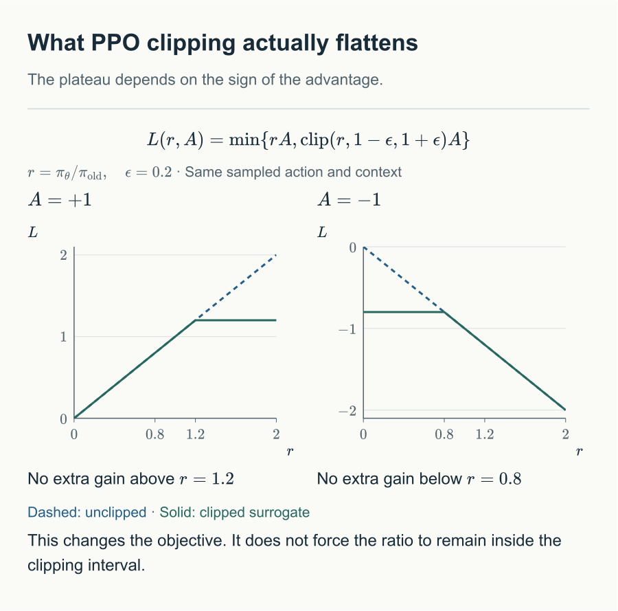
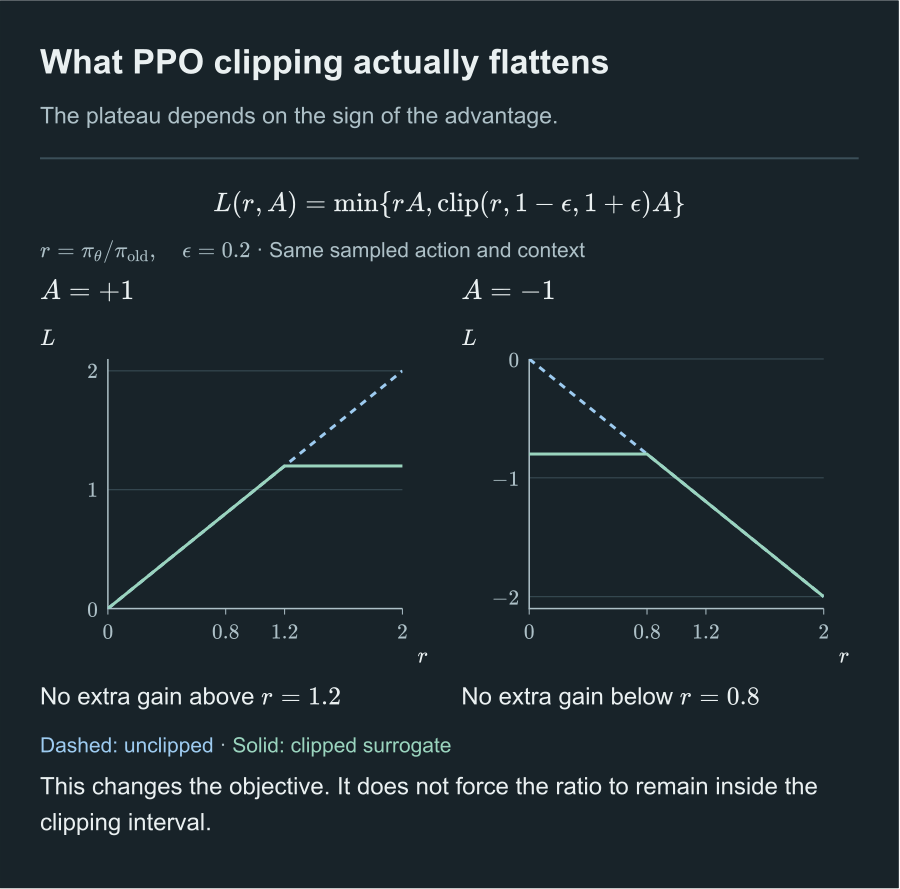
PPO flattens the surrogate on different sides for positive and negative advantages; it does not enforce a hard bound on the ratio.
The Algorithm
Everything assembles into a loop with one extra layer compared to REINFORCE: an inner loop that spends the same batch repeatedly.
Algorithm 1 PPO with the Clipped Objective
Require: initial policy parameters , clip width , epochs , step size
1:repeat
2: // freeze the distribution the batch comes from
3:collect batch of trajectories by running
4:compute for every timestep in
5:for to do
6:for all minibatches do
7:
8:end for
9:end for
10:until converged
Typical values are between and , and .
Step 1 is where the chapter's whole argument is discharged. Freezing fixes the distribution the batch is understood to come from, and it stays frozen for all epochs while moves away from it. At the start of the inner loop , so everywhere and the first update is exactly the policy-gradient step of the previous chapter. Every subsequent update is reuse, paid for with the ratio and policed by the clip. When the loop ends, is refreshed and the batch discarded.
The gain is the factor . One round of generation now funds epochs of updates rather than one, and in a setting where generation dominates the cost, that is close to a factor of in wall-clock efficiency.
What Clipping Actually Guarantees
The story assembled so far is tidy: reuse needs locality, locality is measured by , and clipping keeps the ratio in a band around one. It is worth being precise about how much of that last step is actually true, because the tidy version is false and widely believed.
The clipped objective does not constrain to . It cannot: is an objective, not a constraint set, and the proposition above says only that its derivative with respect to that sample's own ratio vanishes outside the band.
The parameters are shared. The gradient actually applied is a sum over the whole minibatch,
and a sample whose own has been masked to zero still has its moved, because every other sample in the minibatch is pulling on the same . Masking a sample's gradient stops the objective from pushing that sample further out; it does nothing to stop the sample from being carried further out by its neighbours. And nothing anywhere projects a stray ratio back: once is outside the band, the clip's only response is to stop caring.
Across epochs of minibatch updates, ratios therefore drift out of the band routinely, and is bounded by no function of .
The consequence for how this chapter should be read is worth stating without hedging. The trust-region reading of PPO, in which delimits a region the policy is kept inside, is a story about the objective's shape, not a theorem about the algorithm's behaviour. What is true is weaker and still useful: clipping removes the reward for large policy changes, so the optimizer has no incentive to seek them, and in practice the ratios mostly stay near one, mostly. The gap between "has no incentive to" and "cannot" is why implementations monitor during training and stop the inner loop early when it grows too large, a safeguard that would be redundant if clipping did what it is usually described as doing.
PPO takes an exact identity (importance sampling), which licenses reuse, and pays for it with a variance that grows as the policies separate, plus a surrogate whose accuracy is guaranteed at a single point. It then controls the separation with a per-sample, one-sided, first-order gradient mask that guarantees nothing, and it works well.
This is not a defect in the exposition. It is what PPO is: a heuristic with an excellent empirical record, wearing the vocabulary of a trust region it does not implement. A reader who can say precisely which parts are theorems (the identity, the variance formula, the first-order agreement, the gradient mask) and which parts are hope (that the mask keeps small) understands PPO better than one who has been told the tidy version.
Extension: The Penalty Variant
The paper that introduced PPO proposed two ways to keep the policy near , and this chapter has developed only one of them. The other replaces the clip with an explicit penalty:
with adapted between iterations: raised when the measured overshoots a target, lowered when it undershoots. It is the more direct expression of the idea, since it penalizes exactly the quantity the previous sections identified, and it does not pretend that bounding a ratio bounds a divergence.
It is nonetheless not what the field settled on. The clipped variant performed better in the original comparison and is simpler to tune, having one constant instead of a controller with a target and an adaptation rule, and essentially all subsequent work means the clipped objective when it says PPO. The penalty variant is included here as a pointer rather than a topic: readers who want it will find it in the original paper and in Easy RL, Chapter 5.2.1.
Further Reading
This chapter assumed the policy-gradient identity, the log-derivative trick, the trajectory factorization, and the advantage estimator, all from Policy Gradient, and the value functions of Return, Value, and the Bellman Equation.
The divergence introduced here returns as a load-bearing object rather than a diagnostic in the chapters on preference-based methods, where a penalty against a fixed reference policy, rather than against the previous iterate, becomes part of the objective being optimized.
References
- Schulman, J., Wolski, F., Dhariwal, P., Radford, A., & Klimov, O. (2017). Proximal Policy Optimization Algorithms. arXiv:1707.06347
- Datawhale Easy RL, Chapter 5
- OpenAI Spinning Up: Proximal Policy Optimization
Comments