What Makes a State a State
The previous chapter left “maximize expected cumulative reward” not yet well-posed, and named the missing piece: a structural assumption about states. This chapter supplies it, and then builds the standard environment model of reinforcement learning on top of it in three rungs.
Start with the assumption itself. Before any environment model can be built, “state” needs a precise meaning. Not every summary of the past deserves to be called a state; the Markov property is the condition that decides which ones do.
A state is Markov if, conditioned on , the future is independent of the entire past history:
When actions are involved, the same statement conditions on the action as well:
Plainly: given the current state, the future is conditionally independent of the past.
This is exactly the notion of a sufficient statistic from classical statistics, applied to time instead of to a sample. A sufficient statistic for a parameter is a summary of data that loses no information relevant to inferring that parameter. Everything else in the raw data is noise once you have it. A Markov state is a sufficient statistic for the future: it is a summary of history that loses no information relevant to predicting what happens next. This is also, not coincidentally, the same idea that lets physics write down first-order differential equations for dynamical systems. Position and momentum are a Markov state for classical mechanics precisely because they screen off the system’s entire history from its future evolution. “Find a state” and “find a sufficient statistic for the future” are the same problem wearing different clothes.
What It Costs to Do Without
The definition says what the Markov property asserts, and the remark above says what it means. Neither says why anyone would assume it. The usual answer, that it makes the mathematics tractable, undersells the situation: without it, the model is not merely inconvenient to work with, it is not representable and not learnable at all. That claim can be made exact by counting.
Let the state space be finite with , and fix a horizon . A transition model that conditions on the entire history requires
free parameters. A transition model that assumes the Markov property requires , independent of .
At time , the history ranges over distinct values. Each one indexes its own distribution over the possible next states, and a distribution over outcomes has free parameters, since the probabilities are constrained to sum to one. Time therefore contributes parameters. Summing over the transitions and evaluating the geometric series for ,
Note these are genuinely different tables: the histories have different lengths at different , so nothing forces the model at one timestep to share parameters with another.
Under the Markov property, for every , so all tables collapse onto a single stochastic matrix. It has rows, each a distribution over outcomes, hence free parameters, and has left the expression entirely.
The gap this opens is not a constant factor. Take a grid world, so , with episodes of steps, which is a small problem by any standard:
| Conditioning on | Free parameters | Grid world, , |
|---|---|---|
| The entire history | ||
| The last states | ||
| The last state only (Markov) |
The full-history model needs on the order of numbers. The observable universe contains roughly atoms. The request is not expensive, it is not a request that can be addressed by any physical amount of memory, and the Markov model answers the same question with numbers, which fits comfortably in a cache line’s worth of pages.
Storage is the easier objection to state and the less serious one. Suppose memory were free. The parameters would still have to be estimated from data, and here the full-history model fails in a way no hardware can rescue.
To estimate for a history by counting frequencies, the learner must visit many times. But within a single trajectory, each history prefix occurs exactly once, by construction: a trajectory passes through each of its own prefixes one time. So visits to a given length- history can only be accumulated across trajectories, and there are histories competing for them. Seeing each length- history even once, let alone often enough to estimate a distribution conditioned on it, requires on the order of trajectories.
The Markov property changes what the data is pooled over. Every visit to state , at any timestep, in any trajectory, whatever came before it, is evidence about the same row . The requirement collapses from “visit this exact history repeatedly” to “visit this state repeatedly,” and the latter is satisfied constantly by ordinary interaction. This is why the Markov property is an enabling assumption rather than a convenience: it is the thing that makes the transition model estimable from a finite amount of experience.
Full history and last-state-only are the two extremes of a spectrum. An order- Markov model conditions on the last states, costing parameters, and recovers the ordinary Markov property at . The table above prices the dial: on the grid world, costs parameters, costs , costs about , and is already past . Every additional remembered step multiplies the model by another factor of .
This is the bill for the history-augmentation fixes named at the end of this section. Frame stacking is exactly an order- model, and the reason it stacks four frames rather than four hundred is visible in that geometric growth, not in any deep principle.
The counting above assumes the model is stored explicitly, as a table indexed by history. Replacing the table with a function approximator changes the storage arithmetic: a network mapping a history to a next-state distribution has whatever parameter count its architecture has, not .
It does not repeal the statistical argument. The approximator still has to learn the mapping from data, and the data still contains each long history at most once per trajectory. What function approximation actually buys is generalization across histories: an assumption, implicit in the architecture, that similar histories have similar futures. That is not an escape from the problem in this section. It is a different structural assumption doing the same job the Markov property does here, chosen for the same reason, and it should be recognized as an assumption rather than mistaken for their absence.
Being Markov is not automatic. It is a property the state representation either has or lacks, and getting it right matters:
A Markov state must contain everything task-relevant needed to predict the next-state distribution, the immediate reward, and, once actions exist, the consequences of every available action. If the state representation omits important history, two identical-looking states may in fact have different futures. Value functions and policies learned from such an insufficient state can be wrong in a structural sense: the agent is solving a partially observed problem while its algorithms assume a fully observed one.
If the current observation is not Markov, common fixes include augmenting the state with history, frame stacking, an RNN or other hidden state, learning an explicit belief state, or reformulating the problem as a POMDP (partially observable MDP). The deeper issue is never just that computation becomes large. It is that the state representation is structurally insufficient, so whatever value function or policy gets learned from it may not even be well-defined for the true underlying process.
Everything from here on assumes the property holds. The three rungs below are what can be built once it does, added one ingredient at a time, because each addition changes what questions the model is capable of asking.
Rung One: State Transition Alone
The simplest object satisfying the Markov property is a system with a state space and a rule for moving between states, and nothing else.
A Markov process is a system that moves randomly between states while satisfying the Markov property. It is written as the pair
where is the state space and is the transition probability, : if the current state is , the system moves to state with probability .
There is no agent here, and no reward. The world simply evolves on its own, according to , and nothing in the model asks whether any particular state is good or bad. It only describes how states change over time. In compressed form: MP = state transition, and nothing else.
Rung Two: Adding a Notion of Good
The first rung of structure to add above a bare Markov process is a scalar judgment of outcomes (a reward) together with a way to aggregate rewards over an unboundedly long future.
A Markov reward process is a Markov process with reward and discounting added:
where is the reward function and is the discount factor. In compressed form: MRP = MP + reward + discount.
Having reward is what finally lets the model ask a question a bare Markov process cannot: starting from state , how much long-term reward should we expect? Answering that precisely requires two more pieces of machinery, the discounted return and the value function, which are substantial enough to deserve their own chapter. For now, the important structural fact is narrower: an MRP still has no agent action. The system transitions according to , exactly as in a bare Markov process; reward is commentary added on top of a transition process that nothing is steering.
Rung Three: Adding Control
The final rung is the one that turns a passively evolving, scored system into something an agent can actually act inside of.
A Markov decision process is a Markov reward process with actions added:
where is the action space. In compressed form: MDP = MRP + action.
Adding changes the transition and reward functions themselves, not just their interpretation. Where a Markov process or Markov reward process transitions according to , a Markov decision process transitions according to
and reward is typically written or rather than . The future is no longer just the world evolving by itself with a running score attached; it is shaped by which action the agent chooses at every step.
That change has an immediate consequence, and it is the reason this rung is not merely the previous one with an extra letter in the tuple.
Once actions exist, a state’s value alone is no longer enough to compare actions against each other. Two value functions are needed: the state-value function , asking starting in state and following policy , what long-term return should we expect?, and the action-value function , asking starting in state , first taking action , and then following , what long-term return should we expect?
This split between and , and the recursive Bellman equations that relate them to each other and to reward, is what the next chapter is about. This one stops at the point where the question becomes precisely askable.
The Ladder, Compressed
| Model | State transitions | Reward | Action |
|---|---|---|---|
| Markov process (MP) | yes, | no | no |
| Markov reward process (MRP) | yes, | yes, , discounted by | no |
| Markov decision process (MDP) | yes, | yes, | yes, |
Read as plain language: an MP is a world that moves by itself. An MRP is a world that moves by itself, where each step also carries a score. An MDP is a world where an agent chooses actions, the world responds, and each step still carries a score. Reinforcement learning, in essentially all of its classical formulations, is the study of what to do once you are standing at the top of this ladder.
The ladder is also worth remembering downward, not just upward. Later chapters repeatedly collapse an MDP back down a rung on purpose: fixing a policy and averaging the action out turns an MDP back into the MRP it induces, which is precisely the trick that makes policy evaluation an already-solved problem rather than a new one.
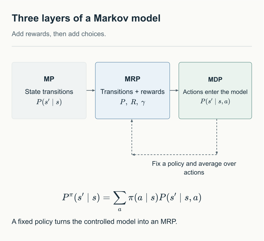
Adding rewards gives an MRP; adding actions gives an MDP. Fixing a policy averages over actions to recover an MRP.
Comments