Two Words That Get Conflated
“Reward is the expected long-term reward” is a sentence that sounds almost right and is actually wrong in a way worth dwelling on.
Reward is one-step feedback: a single scalar handed back by the environment after one transition. Return is accumulated future reward from a given point onward, a sum, not a single number. The chain runs in one direction only: reward aggregates into return, and return in expectation becomes value. This chapter walks that chain end to end, and the payoff is that the Bellman equation, usually presented as a block to memorize, arrives as a consequence of one small lemma proved in the first section.
The discounted return from time is
For a finite horizon ending at ,
If , the return collapses to the very next reward, .
The discount factor is not a minor tuning knob; it is what makes well-defined at all in the general case. An unweighted infinite sum of rewards has no reason to converge, and many environments genuinely admit unboundedly long or cyclic trajectories. Discounting also encodes something more substantive than convergence bookkeeping: it says that reward further in the future counts for less, which is a reasonable stance whenever the future is less certain than the present, or when a task simply prefers reward sooner rather than later. As moves toward , the agent becomes almost entirely near-sighted, valuing only immediate reward; as moves toward , it weighs the distant future almost as heavily as the present.
This also retires the loose end left open at the end of the first chapter. “Cumulative reward” over an unboundedly long future is now a convergent quantity, and it has a name.
The return has a structural property that everything downstream depends on: it can be split into what happens on the very next step, and what happens after that.
The middle step only factors out of every term but the first; the result inside the parentheses is, by definition, .
This one-line identity is the entire mathematical content of the Bellman equation, before any expectation or environment structure gets involved. It is worth keeping in view for the rest of the chapter: every equation below is this lemma wearing progressively more clothing.
Two Value Functions
A value function estimates expected long-term cumulative reward, not just immediate reward. The Markov ladder already flagged why one such function will not be enough once actions exist: different actions available from the same state can lead to different futures. Here is that claim, made precise.
Under a fixed policy , the state-value function is the expected return starting from state and following thereafter:
The action-value function is the expected return starting from , taking action first, and following afterward:
| Function | Evaluates | Includes first action? |
|---|---|---|
| state | no | |
| state-action pair | yes |
The difference is exactly whether the first action is dictated by the policy or fixed by hand, and that difference is precisely what makes useful for comparing candidate actions against each other, while only ever evaluates a state as a whole.
averages the return over trajectories starting at under ; the first action in such a trajectory is itself distributed as . Conditioning on the value of that first action and applying the tower property,
Keep this proposition in hand. It is one of the two halves the Bellman expectation equation gets assembled from a few paragraphs below.
Value Now, Reward Plus Value Later
Now push the recursion lemma through the expectation. Take the MRP case first, where and no actions are involved. Because the return satisfies , so does .
Starting from the definition and applying the one-step recursion lemma:
The first term is exactly , the expected immediate reward from , by definition of the reward function. The second term needs one more step: is an expectation over the next state of the expectation of given that next state. This is the tower property (law of total expectation), conditioning on inside the outer expectation over :
The last equality holds because is, by definition, , the process has no memory beyond the current state, by the Markov property. This step also silently uses that the dynamics are time-homogeneous: does not depend on itself, only on the state, so the value “one step into the future” and “at any other time” are computed by the same function . This is a standing assumption throughout this series, not something the Markov property alone guarantees. Substituting both pieces back in gives the claimed equation.
Read in words: value now equals immediate reward plus discounted expected value one step later. That sentence is the entire content of the Bellman equation; the sum over is just what “expected value one step later” means once you write out the expectation explicitly. Every Bellman equation in reinforcement learning, expectation, optimality, MRP, MDP, tabular or function-approximated, is a variation on this same one-line idea, because it is a direct consequence of the return satisfying and nothing else.
From MRP to MDP: Two Halves of the Same Backup
The proposition above already proved , half of the relationship between and . The other half is a direct MDP analogue of the MRP Bellman equation just derived, with the first action fixed.
The argument is identical to the MRP Bellman equation’s proof, with every transition and reward now conditioned on the fixed action as well as the state . Fixing turns the first step back into an ordinary MRP-style backup, which is why the proof is not repeated here.
Composing the two halves, substituting the action-value backup into the state-value average, gives the Bellman expectation equation:
This equation is usually presented as a single block to memorize. Built up this way, it decomposes into two independent, individually obvious facts: value-from-action-value is just the definition of expectation over the first action, and action-value-from-state-value is just the MRP Bellman equation with the action held fixed. The “expectation” in “Bellman expectation equation” refers to exactly one thing: the average over actions sampled from , layered on top of the same recursive structure derived from .
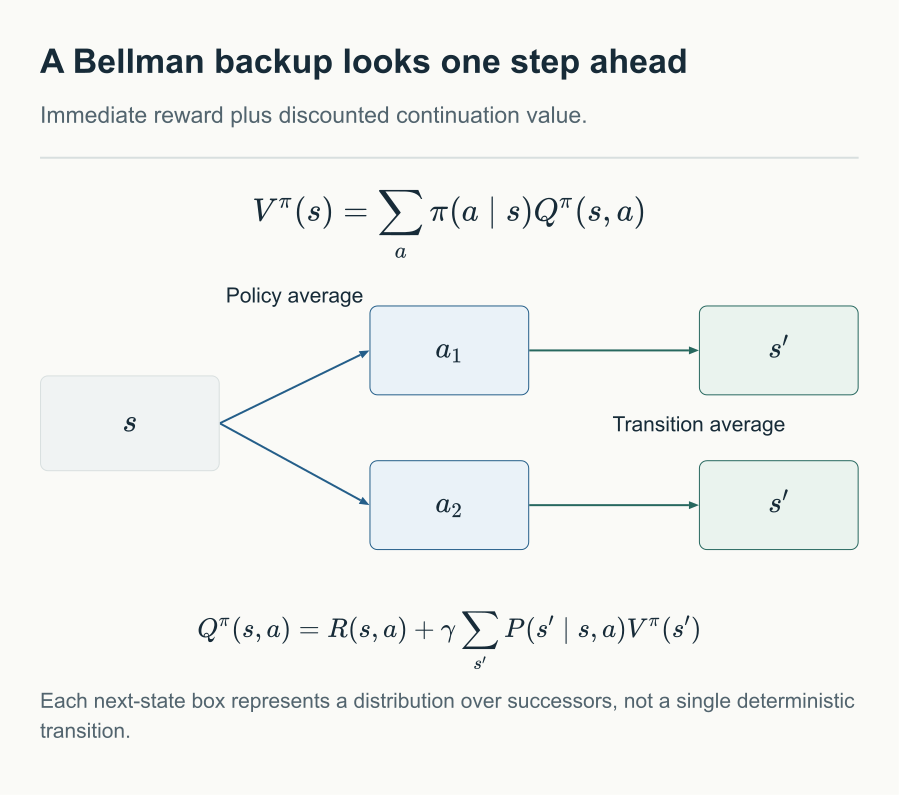
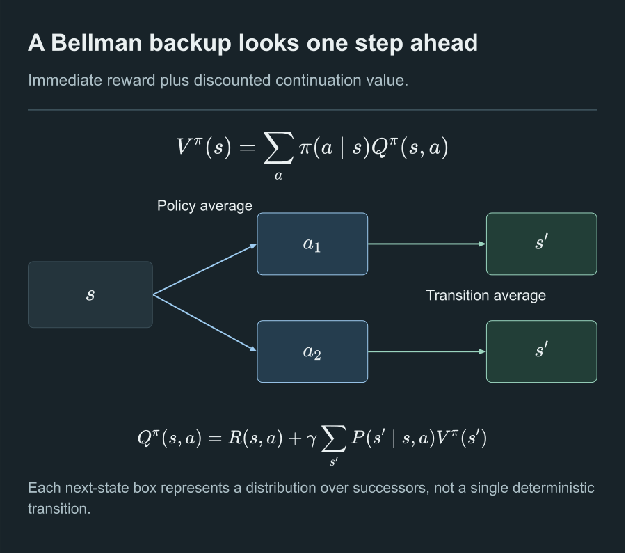
The state value averages over policy actions; each action value averages over possible successor states.
From Evaluating a Policy to Finding the Best One
Everything so far evaluates a fixed policy , this is the prediction problem. Control asks a different, harder question: what is the best possible value achievable at each state, over every policy at once?
Richard Bellman’s original 1957 statement of the idea behind all of this is worth quoting directly, because it is the actual justification for replacing an average over actions with a maximum: an optimal policy has the property that, whatever the initial state and initial decision are, the remaining decisions must constitute an optimal policy with regard to the state resulting from the first decision. Optimality is self-similar across time: the tail of an optimal plan is itself an optimal plan for the sub-problem it starts. This is what licenses solving a problem with an unboundedly long horizon by a local, one-step recursive equation at all. Without it, there would be no reason to expect that a short-sighted, one-step-at-a-time backup could ever assemble into a globally optimal policy.
These equations are not a separate derivation from the Bellman expectation equations above, they are what the expectation equations become once is required to be optimal. By the principle of optimality, an optimal policy must place all of its probability mass on whichever action maximizes at every state; averaging over a distribution that is entirely concentrated on its own maximizer is the same as just taking that maximum. The is the trace left behind by optimizing over itself, not a new assumption bolted onto the earlier recursion.
Formula Ownership Rule
With three families of Bellman equation now on the table, a quick rule settles which one is in front of you:
| Pattern in the equation | Which Bellman equation |
|---|---|
| No action term at all | Markov reward process |
| Action term, averaged with a fixed | Policy evaluation / prediction |
| Action term, combined with or | Control / optimality |
Further Reading
This chapter derives the recursive structure but stops short of turning it into an algorithm. A Bellman equation is an identity, a true statement a value function must satisfy, and not yet a procedure for computing one. Planning with a Known Model closes that gap, by proving the operators behind these equations are contractions and therefore that repeatedly applying them converges.
The value functions built here are also exactly the objects that value-based and actor-critic methods reuse later: the baseline and advantage-function machinery in Policy Gradient is , , and from this chapter, put to work reducing the variance of a different kind of estimator.
References
- Datawhale Easy RL, Chapter 2
- OpenAI Spinning Up: Part 1, Key Concepts in RL
- Bellman, R. (1957). Dynamic Programming. Princeton University Press.
Comments