From Equation to Iteration
A Bellman equation is a recursive identity, a true statement a value function must satisfy, and not yet a procedure for computing one. This chapter closes that gap, and does it three times: for evaluating a fixed policy, for improving one, and for collapsing both into a single backup.
Everything here assumes the environment’s dynamics and are fully known in advance. That assumption matters enough to name up front: this is planning, not yet learning from sampled experience. The first chapter drew that line as the model-based/model-free split, and this chapter lives entirely on the known-model side of it. The last section returns to what happens when the assumption is dropped, which is the reason the rest of this series exists.
One idea carries all three algorithms, and it is worth stating before any of them: each is a fixed-point iteration of an operator that turns out to be a contraction. Once that is established, existence, uniqueness, and convergence all arrive together from a single theorem, and never have to be argued again.
Policy Evaluation
Given a Markov decision process and a fixed policy , policy evaluation is the problem of computing (or ) for every state. This is the prediction problem: how good is this given policy? Not yet the control problem of finding a better one.
Fixing collapses the MDP back down a rung on the Markov ladder: averaging the action out with turns an MDP into the Markov reward process it induces,
and is exactly the value function of that induced MRP. This is a useful thing to notice, because it means policy evaluation is not a new problem: it is the same fixed-point equation from the previous chapter, just restricted to one fixed policy at a time.
Define the operator acting on any function by
The Bellman expectation equation is now a one-line statement: is a fixed point of , i.e. . Restating the equation as a fixed-point condition on an operator is what makes its computability provable, not just plausible.
For any two functions , measuring distance by the sup-norm ,
For any state ,
since the reward terms cancel. Bounding each difference by and pulling that bound out of both sums,
Both and are probability distributions, so both inner and outer sums equal , leaving . This bound holds for every , hence it holds for the maximum over on the left-hand side as well.
This is where the payoff arrives. is a -contraction with on , which is a complete metric space. The Banach fixed-point theorem then applies directly: has a unique fixed point, and starting from any initial guess , the sequence converges to that fixed point, at the geometric rate . This single fact is simultaneously the reason the Bellman expectation equation has a unique solution at all, and the reason repeatedly applying it as an update rule is guaranteed to find that solution.
Initialize arbitrarily. Repeat, for ,
until stops changing appreciably. The lemma above guarantees .
From Knowing a Policy’s Value to Improving It
Knowing is not the same as knowing whether is any good. The next question is how to use to produce a strictly better policy, and, remarkably, a purely greedy, one-step-lookahead rule turns out to be enough.
Given , the greedy policy with respect to it is
That this greedy policy is never worse, and is strictly better whenever there was any room to improve, is not obvious on its face, since is defined using only one step of lookahead against a value function that itself already assumes the old policy is followed forever after. The following theorem is the reason it works anyway.
If for every state , then for every state .
Since is an average of over , it can never exceed the best available action value at , and by construction achieves that best value:
Expanding the right-hand side with the action-value Bellman equation, but with the action fixed to ,
The same inequality, , holds at every state , including each appearing on the right. Substituting it in for replaces the value one step out with the reward earned by following for one more step, plus a still-looser bound two steps out:
where the expectation tracks the environment’s transitions while every action along the way is chosen by . Repeating this substitution inductively times gives, for every ,
Assuming is bounded (true whenever rewards are bounded and ), the tail term as . Taking the limit turns the finite partial sum into the full discounted return under :
If policy improvement produces no change, , then for every , which is exactly the Bellman optimality equation. Since that equation’s solution is unique, , and is an optimal policy.
This corollary is what turns “alternate evaluation and improvement” into a genuine control algorithm with a stopping condition, rather than a heuristic that might loop forever.
Initialize arbitrarily. Repeat, for :
- Evaluate: compute (via iterative policy evaluation, or exact linear-system solution).
- Improve: set for every .
Stop when ; by the corollary above, is then optimal.
Each intermediate in this loop is a genuine, fully-evaluated policy, a meaningful object in its own right, not just scratch work. That property is exactly what the next section deliberately gives up.
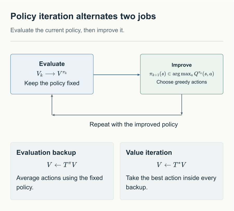
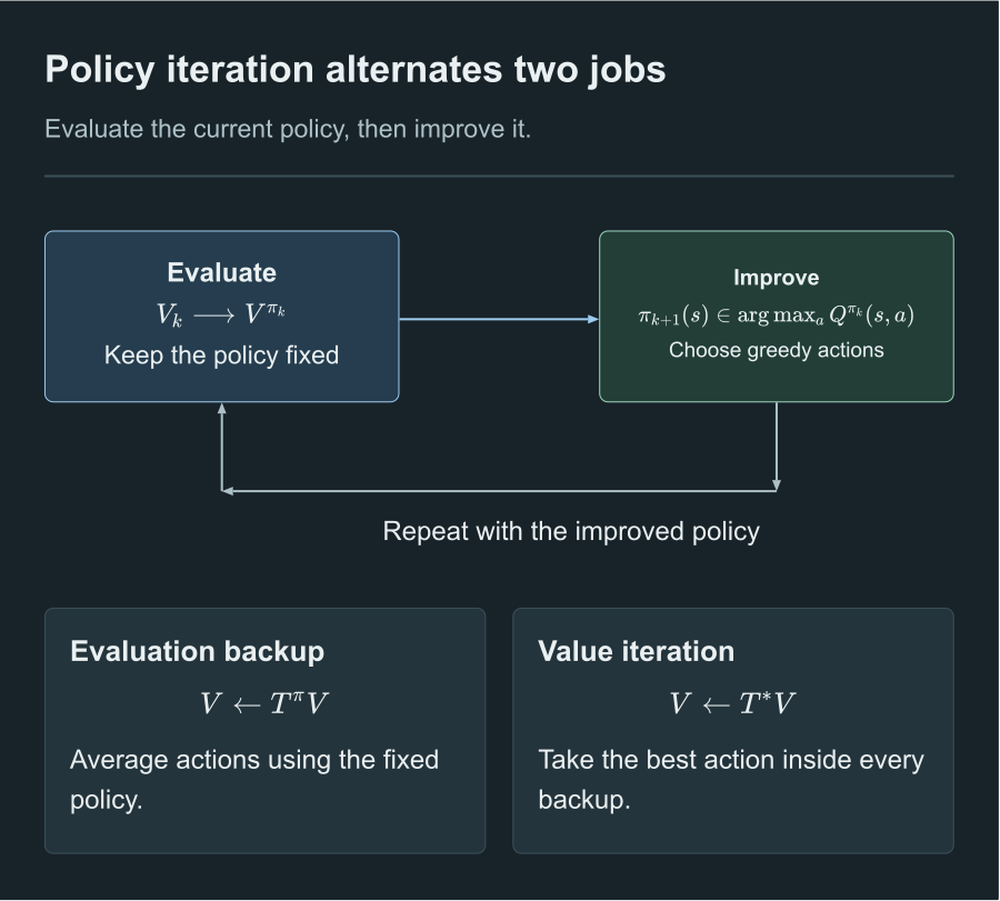
Policy iteration separates evaluation from improvement; value iteration takes the best action inside each backup.
Optimality Backups Without Waiting
Policy iteration pays for its clean intermediate policies with an inner loop: full convergence of policy evaluation before every single improvement step. Value iteration collapses evaluation and improvement into a single backup, applied directly to the optimality equation rather than the expectation equation.
is the fixed point of . This is just the Bellman optimality equation, restated as . Showing is also a contraction needs one extra piece of machinery beyond the proof for above, because a over actions is not linear the way an average weighted by is.
For any two functions on a common finite domain,
Let . Then
using for the middle inequality. Swapping the roles of and gives the same bound on . Combining both directions gives the claimed absolute-value bound.
.
Fix a state and apply the lemma just proved, with and , so that and :
The reward terms cancel inside , leaving for every fixed , exactly the quantity bounded in the proof that is a contraction. The same steps apply verbatim: bound each by and use that sums to , giving for every , and hence . Combining with the first inequality gives for every , hence the same bound on the sup-norm.
Because is a -contraction on the same complete metric space, the Banach fixed-point argument applies again, word for word: has a unique fixed point, and it converges to it geometrically from any starting guess, regardless of whether that guess corresponds to the value of any actual policy.
Initialize arbitrarily. Repeat, for ,
until stops changing appreciably; then extract a policy,
This interactive figure needs JavaScript.
Unlike policy iteration, the intermediate produced along the way need not equal the value function of any policy. They are transient planning estimates being pushed toward , not evaluations of anything an agent could currently be said to be doing. The trade is explicit: policy iteration keeps a meaningful policy at every step at the cost of a full inner evaluation loop; value iteration runs one backup per outer step at the cost of intermediate values that mean nothing on their own until convergence.
Where Planning Stops Being Enough
Every method in this chapter assumed the transition model and reward function were fully known in advance. That is what made backing up an exact expectation, or an exact maximum, over next states a well-defined computation at all.
The moment that assumption is dropped, and the environment must be interacted with and sampled from rather than consulted as a known function, none of these algorithms are directly computable, since none of them can evaluate without knowing . Notice how total the failure is: it is not that the algorithms get slower or less accurate, it is that a single term in every one of them stops being writable.
This is exactly the gap that sampling-based methods exist to close: estimate the same underlying quantities, returns and values, from rollouts, when a model is not available to back up against directly. Policies as Probability Distributions builds the object those methods optimize, and Policy Gradient derives how.
References
- Datawhale Easy RL, Chapter 2
- Bellman, R. (1957). Dynamic Programming. Princeton University Press.
- Sutton, R. S., & Barto, A. G. (2018). Reinforcement Learning: An Introduction (2nd ed.), Chapter 4.
Comments