From Decision Rule to Probability Distribution
A policy answers one question: given state , which action should the agent take? The simplest possible answer is a function.
A deterministic policy maps each state directly to one action:
Given a fixed parameter vector , the same state always produces the same action.
This is enough to define behavior, and it is often how a deterministic policy is actually implemented, for instance as a small multilayer perceptron mapping an observation vector directly to an action vector, with no sampling step and no probability distribution involved anywhere. But a purely deterministic map has a structural weakness already visible from an earlier note in this series: it cannot explore. If always returns the same action from the same state, the agent has no built-in mechanism for trying alternatives to find out whether they are better. Exploration has to be bolted on from outside, as explicit noise added after the fact.
A stochastic policy defines a probability distribution over actions, conditioned on the state:
Sampling an action from it is written .
Exploration falls out of this definition for free: as long as assigns nonzero probability to more than one action, the agent will, by construction, sometimes try something other than what it currently believes is best. But, and this point is easy to blur, that is only one of two genuinely distinct reasons stochastic policies matter, and the other one turns out to be more consequential for what comes after this note.
The first reason is behavioral: a distribution over actions naturally supports exploration, where a deterministic map does not. The second reason is mathematical, and has nothing to do with exploration at all: turning a decision into a distribution, rather than a single point, is what makes it possible to write down a smooth, differentiable objective over the policy’s own parameters, even when the underlying choice is discrete, or when the quantity being optimized (return) is not differentiable in the action itself. This second reason is why policy-gradient methods need specifically, as a genuine probability distribution with a density or mass function, and not merely “some randomness added to a deterministic policy.” It is the subject of the entire log-derivative trick worked out in the Policy Gradient note.
The concrete shape takes depends entirely on the action space it has to cover, and, as with the value-based methods contrasted earlier in this series, discrete and continuous action spaces call for genuinely different constructions.
Discrete Actions: The Categorical Policy
For a discrete action space , a categorical policy outputs a probability vector
In practice this is implemented exactly like a classifier: a network outputs real-valued logits, and a softmax converts them into the probability vector above.
If the sampled action is , its likelihood is , and, the quantity that will matter for everything downstream, its log likelihood is .
Continuous Actions: The Diagonal Gaussian Policy
A categorical distribution has no meaningful analogue once the action space becomes a continuum. There is no way to output “a probability for every real number.” The standard construction instead outputs the parameters of a continuous distribution.
For a -dimensional continuous action , a diagonal Gaussian policy is
with mean vector and covariance matrix restricted to be diagonal, .
Restricting to be diagonal is a genuine modeling choice, not a mathematical necessity. It says the action dimensions are treated as conditionally independent given the state, for each separately. A full covariance matrix could in principle capture correlations between action dimensions (steering angle and speed moving together, say), but at the cost of parameters and a matrix that must be kept positive-definite throughout training. The diagonal restriction trades that expressiveness for parameters and a positivity constraint that only ever has to be enforced coordinate-by-coordinate.
A standard deviation must satisfy , but a neural network’s raw output is an unconstrained real number. Rather than clip or otherwise hard-constrain the network’s output, the standard move is to have the network output instead, and recover . Since is a bijection, this reparameterization enforces positivity exactly, for free, without ever touching the optimizer’s unconstrained parameter space.
Sampling from this policy uses the same trick in reverse: rather than sampling directly from a distribution whose parameters depend on , first sample parameter-free noise, then apply a deterministic, -dependent transformation to it.
Sample , then set
where denotes element-wise multiplication.
The constructed above satisfies .
Each coordinate is an affine transformation of the standard normal variable . An affine transformation of a Gaussian is Gaussian, with mean and variance transforming as and , so . The coordinates of are independent by construction, and an affine, coordinate-wise transformation of independent variables preserves independence, so the are independent as well, which is exactly .
The log likelihood follows from writing out the diagonal Gaussian density and taking its logarithm.
Actions close to the mean have higher log likelihood; actions far from the mean have lower log likelihood; and a larger both widens the distribution and, visible directly in the formula, flattens the log-likelihood’s sensitivity to how far lands from the mean, in exchange for a constant penalty. Larger trades precision for exploration in dimension , and the log-likelihood formula prices that trade-off explicitly.
Log Likelihood: The Object Policies Actually Optimize
Both constructions above end in the same place: not a probability, but a log probability. That is not a stylistic preference.
Writing rather than does two things at once. First, it turns products of probabilities into sums: a trajectory’s probability under a policy factorizes as a product of per-step probabilities, so its log probability is a sum of per-step log probabilities, which is both more numerically stable for long sequences of small numbers and dramatically easier to differentiate term by term. Second, and more fundamentally, the log likelihood is the exact object the log-derivative trick operates on: is precisely the score function that turns “the return of a sampled action” into a usable gradient signal, without ever needing to differentiate through the environment. That identity, why the gradient of a log probability is the right thing to multiply a return by, is substantial enough to deserve its own derivation, and gets one in full in the Policy Gradient note.
Comparison
| Policy type | Action space | Distribution | Main output |
|---|---|---|---|
| Deterministic policy | continuous or discrete | none | direct action |
| Categorical policy | discrete | categorical | action probabilities |
| Diagonal Gaussian policy | continuous | Gaussian | mean and standard deviation |
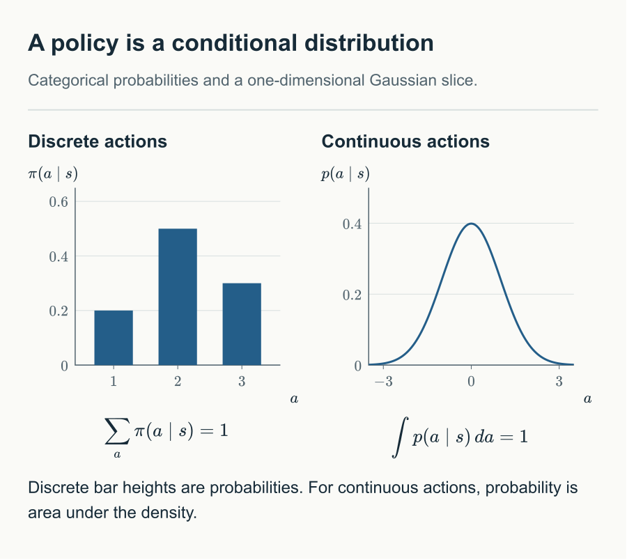
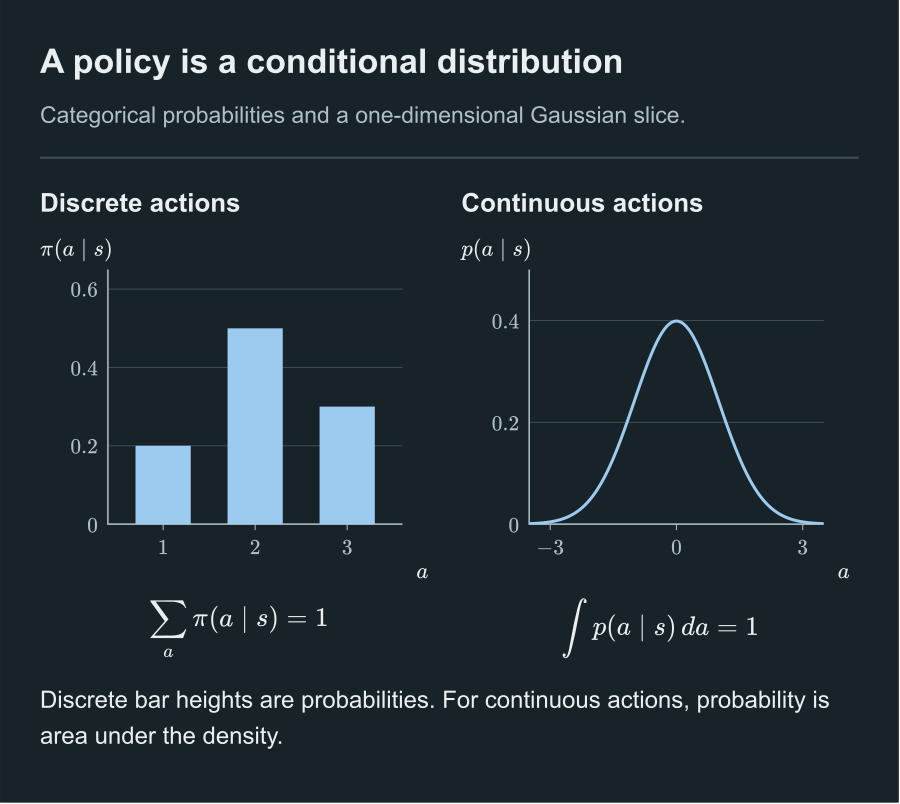
A discrete policy assigns probability to actions; a continuous policy assigns a density whose area gives probability.
Comments