Core Question
Reinforcement learning asks an agent to improve its behavior from experience, without a supervisor that names the correct action at every state. Policy gradient answers this by treating the policy itself as the object being optimized, rather than treating value estimation as a separate problem to solve first and behavior as something extracted from it afterward. The question motivating everything below is:
How can an agent update a policy
so that actions leading to higher future return become more likely?
This sounds simple, but it hides two real difficulties. First, the policy assigns probability to actions, not directly to the returns those actions eventually produce, so there is no ready-made loss to differentiate. Second, the connection between a small change in and the resulting change in expected return runs through an entire trajectory of future states, actions, and rewards, not through a single number computed in one step. The rest of this note is essentially an answer to how that connection can be made precise, and differentiable.
The policy is the object being optimized: a parameterized conditional distribution over actions given a state, controlled entirely by .
Rolling this policy out in the environment for one episode produces a trajectory: the full sequence of states and actions visited from the start of the episode to its end.
Each trajectory carries a trajectory return, the discounted sum of rewards collected along it.
Because the trajectory itself is random (it depends on which actions the policy happened to sample, and on how the environment happened to respond), the quantity actually worth optimizing is not the return of any single rollout, but the expected trajectory return, averaged over every way a rollout under could unfold.
Relationship to Value-Based Methods
Before working through the derivation, it helps to place policy gradient against the family of methods it departs from. Value-based methods (dynamic programming, Monte Carlo control, temporal-difference learning) all work by first estimating how good a state or a state-action pair is, and only afterward deriving behavior from those estimates. Formally, they learn values such as:
and extract a policy from them after the fact, typically by acting greedily with respect to the learned value.
Policy-gradient methods skip that intermediate step entirely. Instead of first learning “how good is this action” and then converting that judgment into a decision rule, they parameterize the decision rule itself and adjust its parameters directly:
The key shift is from “estimate which action is valuable” to “increase or decrease the probability of sampled actions based on return or advantage.” This is not merely a stylistic preference between two equally good options. Section 1 below works through the specific practical problems that value-based extraction runs into, and why parameterizing the policy directly sidesteps them.
Derivation
Here is the expected return of the policy , and is the gradient of the expected return with respect to the parameters at time step . The goal of gradient ascent is to maximize the expected return by iteratively updating the parameters in the direction of the positive gradient.
1. Objective, Notation, and Intuition
Motivation
In a deterministic policy, the policy maps a state directly to an action:
However, policy-gradient methods usually start from a stochastic policy:
which maps a state to a probability distribution over actions. The sampled action is written as:
where the dot means that the action variable is left open: given state , is the full probability distribution over possible actions.
In practice, may be implemented by a neural network, a linear function approximator, or another parameterized controller. The important point is that controls the behavior of the policy, even if the policy is not a simple table.
This distinction matters because policy gradient does not update a value table first. It directly updates the parameters of the policy that assign probabilities to sampled actions.
Earlier dynamic programming, Monte Carlo, and temporal-difference methods usually learn value estimates such as:
In tabular methods, these values are stored explicitly for states or state-action pairs. For example, a tabular Q-learning style update has the form:
This family of methods is conceptually important, but it has practical limitations. A table-based value function is only natural when the state and action spaces are small enough to enumerate. Once states become high-dimensional observations, images, videos, or continuous feature vectors, maintaining a separate value for every possible pair becomes infeasible.
Even when can be approximated by a function, the policy is still usually derived indirectly, for example by choosing:
This indirect extraction can also be awkward in continuous action spaces, where computing may require solving a difficult optimization problem at every decision step. It is also less natural when the desired behavior is a stochastic policy rather than a deterministic greedy action.
Policy gradient addresses this by parameterizing the policy directly and optimizing its parameters:
This is gradient ascent on the expected return objective . It is analogous in form to neural-network gradient descent,
but the sign is different because supervised learning usually minimizes a loss , while policy gradient maximizes expected return .
As its name suggests, policy gradient is an on-policy method for finding an optimal policy , where is the parameter vector of the policy. The goal is still an optimization problem, but we do not directly differentiate a supervised loss against a ground-truth label. Instead, we maximize expected return under trajectories sampled from the current policy.
Consider a complete system for MDP defined by tuple
where:
- is the state space;
- is the action space;
- is the transition probability;
- is the reward function;
- is the discount factor.
The one-step reward function can be written as:
When the action is sampled by the policy,
the observed reward becomes random through the sampled action and the next environment transition. The reward function itself is not directly parameterized by ; changes the distribution over actions and therefore the distribution over trajectories.
The key point is that is a random variable, and the one-step reward function is not usually differentiable with respect to directly.
The return is defined as the total discounted reward from time step to the end of the episode. One common convention is:
Recall the trajectory . The final state is included here because the transition term appears in the trajectory probability; some texts omit it from the shorthand notation.
This allows us to define the return of a trajectory as:
This equality uses the convention that the first sampled reward is and the full-trajectory return is . If a text starts the trajectory at and names the first-step return , the same quantity may be written as .
Different textbooks use slightly different indexing, but they refer to the same discounted sum after reindexing. In this note, action is taken at state , the next reward is , and the reward-to-go from decision time is:
Under this convention, the full-episode trajectory return can be written as:
Other common conventions include:
- starting from and writing ;
- writing reward-to-go as ;
- using lowercase rewards, such as or , instead of ;
- omitting the final state from the shorthand trajectory notation.
The formulas are equivalent only after the indices are shifted consistently. Mixing conventions inside one derivation is the main thing to avoid, including across notes: the interaction sequence sketched in The Reinforcement Learning Problem used the -indexed convention above () for informal illustration, while this note fixes the -indexed convention throughout for the actual derivation.
To sum up, intuitively (using to denote causality):
2. Trajectory Probability
A trajectory is not fixed in advance. It is sampled by rolling out the current policy in the environment, so we write:
where is the trajectory distribution induced by the policy and the environment dynamics.
Here, denotes the whole trajectory distribution, while denotes the probability mass or density assigned to one particular trajectory. The trajectory probability factorizes as:
Here, and come from the environment. The policy terms are the parts controlled by .
This is important because it shows that the expected return is a function of through the trajectory distribution, not through the reward function directly. The expected return objective is:
This is only the definition of expectation. If is a discrete random variable with probability mass function , then for any function :
Taking gives the expected trajectory return above. If the trajectory space is continuous, the summation is replaced by an integral, but the expectation notation means the same thing.
The key point is that is random, and is therefore a random return. However, for a fixed parameter vector , is not a random variable; it is a deterministic scalar objective: the average return of the policy .
From the optimization point of view, policy gradient is trying to solve:
In practice, we do not know how to enumerate all possible trajectories, and the environment dynamics are usually not differentiable through the agent’s parameters. The trick is to estimate the gradient of from sampled trajectories, then apply stochastic gradient ascent:
The derivation below assumes that is not directly parameterized by , the environment dynamics do not depend on , and the trajectory distribution is differentiable with respect to on the sampled support. It also assumes we can exchange gradient and summation or expectation:
For the log-derivative trick, we also need on trajectories where is evaluated.
3. Log-Derivative Trick
We start from the objective in summation form:
Taking the gradient with respect to :
Since the reward function is treated as independent of , the gradient acts on the trajectory probability:
At this point the expression is not convenient, because it asks us to differentiate the probability of a complete trajectory. The log-derivative trick rewrites this term using a positive differentiable function .
For a positive, -differentiable function ,
Read the left-hand side carefully. The outcome is fixed; only the parameter is moving. So means:
if we slightly change , how does the probability or density assigned to this fixed outcome change?
It is not a derivative with respect to . In policy gradient, will later become a sampled trajectory , and we ask how the current policy parameters change the probability assigned to that trajectory.
For a scalar parameter , the chain rule gives:
For a vector parameter , the same statement holds coordinate by coordinate:
Stacking these partial derivatives back into a gradient vector:
Multiplying both sides by gives:
The condition is only there because must be defined. In probability settings, this means we apply the identity on the support where the sampled outcome has nonzero probability or density.
Applying the lemma with :
Here is treated as a fixed sampled trajectory inside the derivative. We are not differentiating the realized states and actions themselves. We are differentiating how much probability the current policy assigns to seeing that complete trajectory.
This identity is commonly called the log-derivative trick. In stochastic-gradient literature, the resulting estimator is also called the score-function estimator, likelihood-ratio estimator, or REINFORCE estimator. It is related in spirit to DDPM and score-based diffusion derivations because both work with gradients of log probabilities. The object is different, though: here the score is a parameter score, , used to estimate without differentiating through the environment. In DDPM-style derivations, the score usually means a data-space score such as , and training is usually presented through denoising score matching plus a reparameterized noising process.
The first line substitutes the corollary above into ; the last line is the definition of expectation.
This is the central policy-gradient identity. It turns an optimization problem over expected return into an expectation of a score function, . In optimization language, this gives us a stochastic gradient estimator: sample trajectories from the current policy, compute the return, compute the score of the sampled trajectory, and move in the estimated ascent direction.
4. Removing Environment Terms
Here, “expand” does not mean Taylor expansion. It means substituting the factorized trajectory probability from the previous section and then using log-product rules.
Recall the trajectory probability:
Taking on both sides:
The only algebra used here is:
Taking the gradient with respect to :
The environment terms do not depend on , so their gradients are zero:
Thus:
Substituting the proposition above into the policy-gradient identity gives:
This is why policy gradient is practical: we do not need to differentiate through the environment transition model. We only need the log probability that the current policy assigned to the actions it actually sampled.
5. Sampled Gradient Estimate
The expectation above is still not computable exactly in most environments.
Sample trajectories by rolling out the current policy,
and approximate the expectation by a sample average:
Then perform gradient ascent:
This is the basic REINFORCE idea: actions that appear in high-return trajectories are reinforced more strongly. Through the policy parameterization and normalization over actions, increasing the probability of some sampled actions also changes the probability mass assigned to other actions.
So the mathematical nature is the same as many stochastic optimization algorithms:
- define an objective ;
- derive a gradient identity;
- replace the true expectation by samples;
- update parameters using stochastic gradient ascent.
6. After the Core Derivation: Credit Assignment
The derivation above gives the cleanest form:
But this assigns the same whole-trajectory return to every action in the episode. That is mathematically valid, but it is noisy. If an action happens early in the episode, using rewards that occurred before the action does not make causal sense for credit assignment.
A common refinement is to replace the full trajectory return with reward-to-go. Using the convention fixed above, this means using the future return after the sampled action, . Unlike the derivation so far, this refinement is a genuine claim: that trading for leaves the estimator’s expectation essentially unchanged, and it is worth actually proving rather than just asserting.
For any state ,
using the log-derivative trick from Section 3 for the second equality, and the fact that sums to for every in the last.
Expand and swap the order of summation:
Fix and split the inner sum at . For , the reward is determined by , states and actions sampled strictly before , so conditioning on the trajectory prefix up to leaves fixed while is still random, and the lemma above gives
Only the terms with survive:
factoring out of the surviving terms. The remaining inner sum is exactly by definition, which gives the claimed identity.
The proposition just proved shows that the exactly unbiased reward-to-go estimator carries an extra weight on the term for time step . The formula below, used throughout the rest of this note (including the REINFORCE box and every downstream advantage-based estimator), instead uses without the factor. This is not an oversight; it is the essentially universal convention in the policy-gradient literature, including Sutton and Barto’s own presentation and OpenAI Spinning Up, both cited in this note’s references. Dropping makes the estimator the exact gradient of a closely related, undiscounted-per-step objective rather than of itself, a small, well-documented bias traded for lower variance and an update rule that weights early and late time steps equally. Since this is a standard, deliberate simplification rather than an error, the rest of this note follows the convention.
This does not change the basic policy-gradient idea. It just gives each sampled action a more relevant measure of future return.
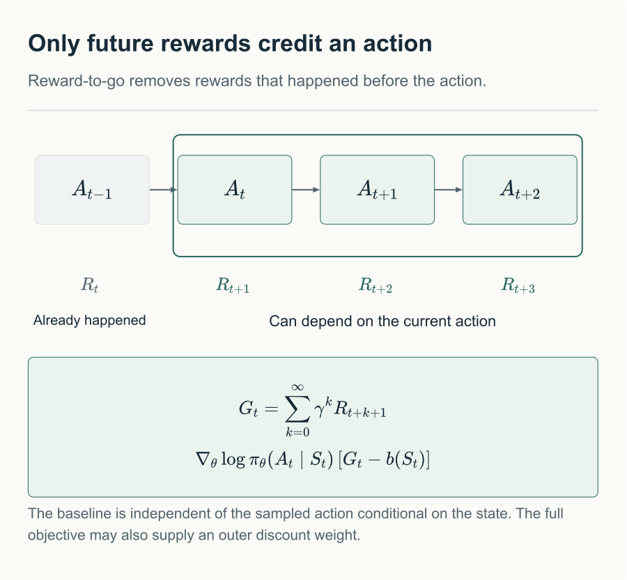
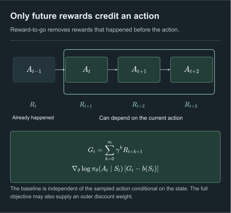
Reward-to-go credits only rewards after the sampled action; a state-dependent baseline can reduce variance.
7. Baseline and Advantage as Variance Reduction
Baseline and advantage are useful, but they are not the core log-trick derivation. They answer a numerical optimization question: how can we reduce the variance of the sampled gradient estimator without changing its expected direction?
A baseline subtracts a state-dependent reference value:
The common choice is .
If the baseline does not depend on the sampled action , it does not bias the policy-gradient direction in expectation.
Subtracting a baseline changes the reward-to-go estimator’s expectation by exactly
using that depends only on and can therefore be pulled outside the inner expectation over , since it does not depend on . The baseline term contributes exactly zero to , for any choice of satisfying this condition.
Writing for the baselined reward-to-go, and choosing as above, is a Monte Carlo estimate of : the sampled reward-to-go is an unbiased (if high-variance) estimate of , since , so estimates .
This is the bridge to actor-critic and PPO. For this note, the main point is only that advantage replaces raw return with a more stable signal for stochastic gradient ascent.
REINFORCE
REINFORCE is the Monte Carlo policy-gradient algorithm corresponding to the derivation above. It samples complete episodes under the current policy and uses their returns to estimate the ascent direction for .
In words: sample trajectories from the current policy, estimate which sampled actions led to good future return, then increase the log probability of those actions by gradient ascent.
PPO Bridge
PPO keeps the policy-gradient idea but constrains how far the new policy can move from the old policy.
Do not study PPO deeply until the policy-gradient derivation is explainable.
Further Reading
This note assumes familiarity with the policy notation built up in Policies as Probability Distributions, and with the value functions and Bellman equations of Return, Value, and the Bellman Equation. The Bellman equation in particular is the useful background for the value-based methods this note contrasts itself against, and , , and are exactly the objects the baseline and advantage sections above put to work. The estimator derived here is on-policy, which means each batch of trajectories funds exactly one update before going stale. Proximal Policy Optimization picks that problem up directly: it buys sample reuse with importance sampling, and spends the rest of its length paying for it.
Comments