The Second Model
Proximal Policy Optimization closed on an objective that reuses a batch times, policed by a clip on the probability ratio:
Everything in that line was accounted for except one symbol: . The chapter treated the advantage estimate as inherited machinery, with , and proved only that subtracting an action-independent baseline leaves the gradient unbiased. It never said where comes from. In the algorithm actually run, it comes from a second neural network.
In full PPO the advantage is computed by Generalized Advantage Estimation, which combines the observed rewards with a learned value function trained alongside the policy by regression toward returns. That is not a small auxiliary. It is a network of roughly the policy's own size, with its own forward and backward pass, its own optimizer state, and its own failure modes. PPO is an actor-critic method, and the critic is the half that this chapter's predecessor quietly folded into the symbol .
So the true cost of a PPO step is two models, not one. The policy is what you want; the critic exists only to supply the baseline that makes the policy's gradient low-variance. It is pure overhead in the sense that it is discarded at the end of training, and it doubles the memory and roughly the compute of every update.
For the domains this series is heading toward, the overhead is compounded by a mismatch. Consider where the reward actually appears.
In the settings that motivate this chapter, a single trajectory is a full generated sequence, and the reward is one scalar delivered at the end: a completion is scored once it is complete, a proof once it is finished. There is no per-step reward, only a terminal one.
A per-token value function is then being asked to predict, at every intermediate token, the expected final score of a sequence that does not yet exist. It must learn to be accurate thousands of tokens before the only supervision signal arrives. This is a genuinely hard regression problem, and it is hard precisely in proportion to how long the generation is, which is to say most where it is needed most. The critic is not only expensive; in the terminal-reward regime it is estimating an awkward object.
The question this chapter answers is whether the baseline can be had without the second network at all.
Can the variance reduction of a value baseline be obtained without learning a value function?
The answer is yes, and it costs samples instead of a model. The rest of the chapter is what that trade buys and what it assumes.
A Baseline You Can Sample
The licence for what follows was proved two chapters ago and is worth restating exactly, because the entire method is one substitution into it.
For any function that depends on the state but not on the action,
so subtracting from the return inside the policy gradient changes neither the gradient's expectation nor its direction.
Pull out of the action-expectation, since it does not depend on , and use the log-derivative identity in reverse:
Multiplying the zero vector by leaves zero.
The best such baseline, the one that removes the most variance, is the state's own value : it centers each return on what the policy expects from that state. PPO learns with the critic. But is an expectation, and there is a second way to obtain an expectation, older than any network.
The value is . In the terminal-reward setting the return from is just the final reward of the trajectory that begins, so
This is an average over the policy's own outputs from . Rather than train a network to predict it, sample it. Draw a group of outputs from , score each, and take the mean:
The same generations that the policy-gradient step consumes are, collectively, a Monte Carlo estimate of the baseline that step needs. The critic's entire job is done by the batch, for free.
This is the whole idea of Group Relative Policy Optimization. Where PPO learns a baseline, GRPO samples one, using a group of completions per prompt precisely so the group has a mean to subtract.
The baseline theorem requires to be independent of the action being scored. The group mean includes the term when it is used as the baseline for output , so it is not strictly independent of , and the estimator carries a bias of order . A leave-one-out mean, excluding , would be exactly unbiased. The method as published uses the full mean for simplicity and takes large enough that the distinction is immaterial. Say it plainly rather than bury it: dropping the learned baseline costs a small, controllable bias, plus generations per prompt instead of one.
The Group-Relative Advantage
Subtracting the group mean gives a centered reward. GRPO takes one further step and normalizes by the group's spread.
For a prompt , let be the rewards of a sampled group of outputs. The advantage assigned to every token of output is
Two things are happening in that ratio, and they have different standing.
The numerator, , is the baseline subtraction of the previous section: the centered reward, an estimate of restricted to the terminal signal. Its meaning is exactly the advantage's meaning from PPO, an output scored relative to the policy's own average on this prompt, positive for above-average completions and negative for below. The sign is a comparison, not an absolute score, just as before.
The denominator, , is not part of that argument.
Dividing by rescales each prompt's advantages to unit variance before they enter the gradient. Its purpose is practical: prompts differ in how spread out their rewards are, and without normalization an easy prompt with tightly clustered rewards and a hard prompt with widely scattered ones would contribute gradients of very different magnitude for no principled reason. The normalization puts them on a common scale, acting as a per-prompt adaptive step size.
It is not, however, part of the unbiased-baseline story. Multiplying an advantage by the positive scalar preserves its sign and the ordering within the group, but it does reweight how much each prompt pulls on : prompts with low reward variance are amplified. This is a deliberate heuristic, not a theorem, and later analyses have noted it introduces a mild bias toward such prompts. For this chapter it is enough to keep the two parts separate: the numerator is the baseline the previous section justified; the denominator is a scaling choice layered on top.
Every token of receives the same , because the reward is terminal: there is one scalar for the whole output, and it is broadcast to each token that helped produce it. This is credit assignment at its bluntest, every token in a good completion is reinforced equally, and it is exactly what the terminal-reward structure permits and the per-token critic tried to refine.
When a reward can be given at the end of each reasoning step rather than only at the end of the whole output, the same construction runs with finer granularity: normalize the step rewards across the group, and set each token's advantage to the sum of normalized rewards from that token onward. This recovers some of the within-trajectory credit assignment the terminal signal throws away, without reintroducing a learned value function. It is a refinement of the advantage, not a change to anything else in the chapter, and outcome supervision is the version to hold in mind.
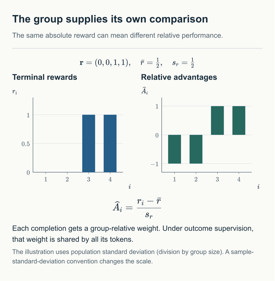
The four-completion example uses population standard deviation. Sample standard deviation changes the scale of the advantages.
The Reference Policy
The critic is gone. One term of the objective is left to build, and it discharges a promise the previous chapter made explicitly.
PPO's KL divergence measured the gap between and , the previous iterate. It was a diagnostic: a quantity watched to decide whether reuse had drifted too far, controlling the locality that importance sampling required. It regularized nothing directly; the clip did the work, and the KL was a monitor.
The KL that enters here is a different object with a different job.
Let be a fixed reference policy, typically the model at the start of fine-tuning. The objective is to maximize the reward while staying close to that reference:
Three differences from PPO's use of KL matter here, and they are easy to conflate:
- The second argument is fixed. does not move as training proceeds; it is a frozen anchor, not the last step's parameters. The policy is kept near where it started, not near where it was.
- It is part of the objective, not a monitor. The term is optimized, its gradient flows into . It is load-bearing in a way PPO's diagnostic KL never was.
- Its purpose is different. PPO's KL guarded the validity of sample reuse. This one guards against the policy exploiting the reward: a learned reward is an imperfect proxy, and a policy free to maximize it will find its blind spots and produce degenerate, high-scoring, useless outputs. Anchoring to keeps the policy in the region where the reward is trustworthy.
is the destination of the whole series' second half. GRPO reaches its maximum by the reinforcement-learning loop this chapter is assembling: sample, score, estimate advantage, step. The next chapter, on Direct Preference Optimization, will take this exact objective and solve it in closed form, discovering that when the reward comes from preferences the loop can be removed entirely. Everything downstream is a statement about how to optimize this one line. Introduced here, it is inherited there.
One smaller design choice is deliberate in the original work and easy to miss. The reward-model literature that PPO fine-tuning grew out of folds the KL penalty into the reward, subtracting a per-token from the score before advantages are computed. GRPO instead adds the KL directly to the loss, leaving the advantage computation to depend only on the reward model's output. The two are not equivalent bookkeeping: keeping KL out of the reward means the group normalization above acts on the clean reward signal, and the divergence is regularized as its own term rather than laundered through the advantage.
Estimating the Divergence
The objective needs , but the expectation defining it ranges over the whole vocabulary at every token and is not computed exactly. It is estimated from the sampled tokens, and the choice of estimator is not obvious, because the naive one misbehaves.
The definition is
. Estimating it by its integrand, a single sample of , is unbiased but has a defect: it is negative whenever a sampled token is more likely under than under , even though the quantity it estimates is non-negative. A regularizer that is supposed to penalize divergence but frequently reports a negative value injects noise of the wrong sign. GRPO uses a better estimator.
Writing for a sampled token, the per-token divergence estimate is
It has exactly the two properties the naive estimator lacks and keeps, together, the one it had.
For every sampled token, , with equality iff at that token. And taking the expectation over ,
Non-negativity. For any the inequality holds, with equality iff (it is the tangent line to the concave at ). Rearranged, , and means the two policies agree on that token.
Unbiasedness. Split the expectation into three terms. The first is
the same "the ratio averages to one" identity used in the PPO chapter, now with the reference in the numerator. The second is
by the definition of KL. The third is the constant . Summing, .
So estimates the right thing on average and never reports a negative penalty. That it is both unbiased and non-negative is the reason it is preferred over the integrand; the extra , which averages to zero, is a control variate that removes the sign problem without touching the mean.
The Objective and the Algorithm
Assembling the pieces, the clipped surrogate of PPO, the group advantage in place of the critic's, and the reference-KL as an explicit term, gives the GRPO objective.
where
is the per-token probability ratio, is the group-relative advantage, and the expectation is over prompts and groups sampled from .
Read against PPO's , the objective is the same clipped surrogate with two edits. The advantage is now the group-relative quantity, no critic anywhere in it. And the term is appended, the reference anchor made explicit. The clipping machinery, and everything the previous chapter proved about what it does and does not guarantee, carries over unchanged: it still only masks each sample's own gradient outside the band, still bounds no divergence by itself. That analysis is not repeated here; it applies verbatim.
The loop is PPO's with the critic's training deleted and a group sample inserted.
Algorithm 1 GRPO with Outcome Supervision
Require: initial policy , reward model , prompts , group size , clip width , KL weight , inner epochs , step size
1: // freeze the anchor for the KL term
2:repeat
3:
4:sample a batch of prompts
5:for each , sample a group
6:score every output:
7: for all tokens of
8:for to do
9:
10:end for
11:until converged
What was deleted is the entire actor-critic apparatus for the value function: no value network, no value forward pass, no value loss, no value optimizer state. In a regime where the models are large enough that holding two of them dominates the memory budget, dropping one is not a marginal saving. What was added is generations per prompt instead of one, which is more sampling but of the cheap kind relative to holding and training a second network, and it is sampling the group approach turns to double duty: the same completions are both what the policy gradient reinforces and what estimates the baseline.
Freezing once at the start is the simplest version and the one to understand first. In practice the reference is sometimes refreshed to the current policy every so often, so the anchor tracks the policy at a slow cadence while tracks it at every step. This is a knob on how much total drift from the starting model is permitted, and it does not change anything in the objective above; it only says which frozen copy plays .
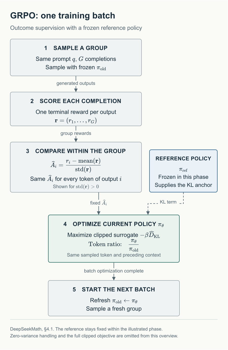
The flow below summarizes one outcome-supervised batch. The behavior snapshot generates the group, is optimized, and stays frozen within the illustrated training phase.
Application: Reinforcement Learning on a Language Model
The chapter so far is agent-agnostic. Nothing above mentions language: it needs a state, a policy over actions, a terminal scalar reward, and a reference policy, and a robot controller with a sparse end-of-episode reward would fit the same objective. But the setting where GRPO is usually first met, and the one that motivated its terminal-reward framing, is post-training a language model, and it is worth spending a section reading the abstractions back onto that case, because the mapping is where most of the confusion lives.
Four questions carry the translation.
How does the Markov decision process transfer? The correspondence is exact once the pieces are named:
| RL object | Language-model instantiation |
|---|---|
| initial state | the prompt |
| action | the next token |
| state | the prompt plus tokens so far, |
| transition | deterministic: append to the context |
| trajectory | the full completion |
| terminal reward | one score for the finished completion |
The transition is the special feature: appending a token to a context is deterministic, so all the environment's stochasticity that the PPO chapter carried, , collapses. The only randomness in a rollout is the policy's own sampling of tokens. The generation is the trajectory.
What is the action space, and what supplies the reward? The action space is the vocabulary, tens of thousands of tokens, and the policy is literally the language model's next-token distribution, the softmax over that vocabulary. There is no separate policy network to build; the model being fine-tuned is the policy. The reward is not part of the environment, as it would be in a game. It is supplied by a separate learned model , and the humans whose judgment it encodes are not in the loop.
How are tokens treated inside the objective? Every mechanism in the objective is per-token: a ratio , a clip, a KL estimate, one for each token position. But the reward is per-sequence, delivered once. Outcome supervision resolves the mismatch by broadcasting the single normalized reward to every token of the completion, so is constant across within an output. This is the same fact that made the per-token critic awkward, seen from the other side: because the signal is terminal, a constant-per-sequence advantage is what there is to work with, and the group baseline supplies it without pretending to per-token resolution the reward does not have.
How does human preference enter? Not through the loop, but through , which is trained once, beforehand, on human comparisons. This is the piece that turns "reinforcement learning" into "reinforcement learning from human feedback," and it is worth making precise, because the reward model built here is exactly the object the next chapter dismantles.
Humans are shown a prompt and two completions and asked which they prefer, yielding a dataset of triples where is the preferred ("winning") completion and the rejected ("losing") one. Under the Bradley-Terry model, the probability that is preferred is assumed to be
where is the logistic function. The reward model is trained to maximize the likelihood of the observed preferences, i.e.\ to minimize
The model learns a scalar score whose differences reproduce human choices. Only differences are constrained: the Bradley-Terry likelihood is unchanged if a constant is added to every score at a given prompt, so is identified only up to a per-prompt shift, a fact that looks like a technicality here and becomes the load-bearing cancellation of the next chapter.
With the reward model in hand, the three stages and the flow of data among the models look like this:
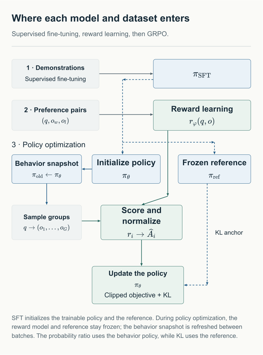
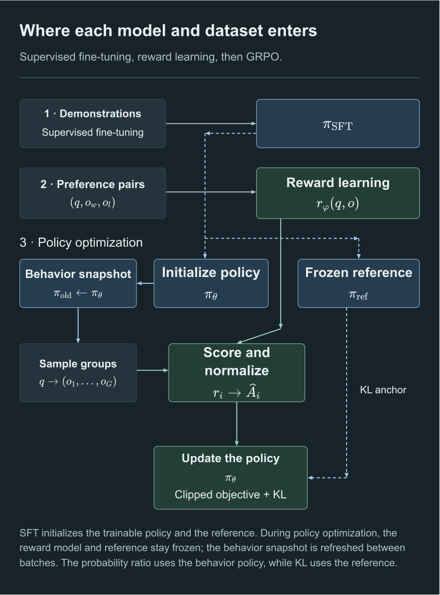
The trainable policy, behavior snapshot, frozen reward model, and frozen reference play distinct roles during this GRPO phase.
The diagram makes the model economy visible. One supervised model is trained and then copied three ways: it seeds the reward model, it becomes the initial policy, and a frozen copy of it is the reference. During GRPO only the policy trains; the reward model and the reference are frozen. The preference dataset touches the pipeline exactly once, at reward-model training, and thereafter human judgment reaches the policy only through 's scores.
And a single rollout, the trajectory the RL objective is defined over, is one left-to-right generation with the score arriving only at the end:
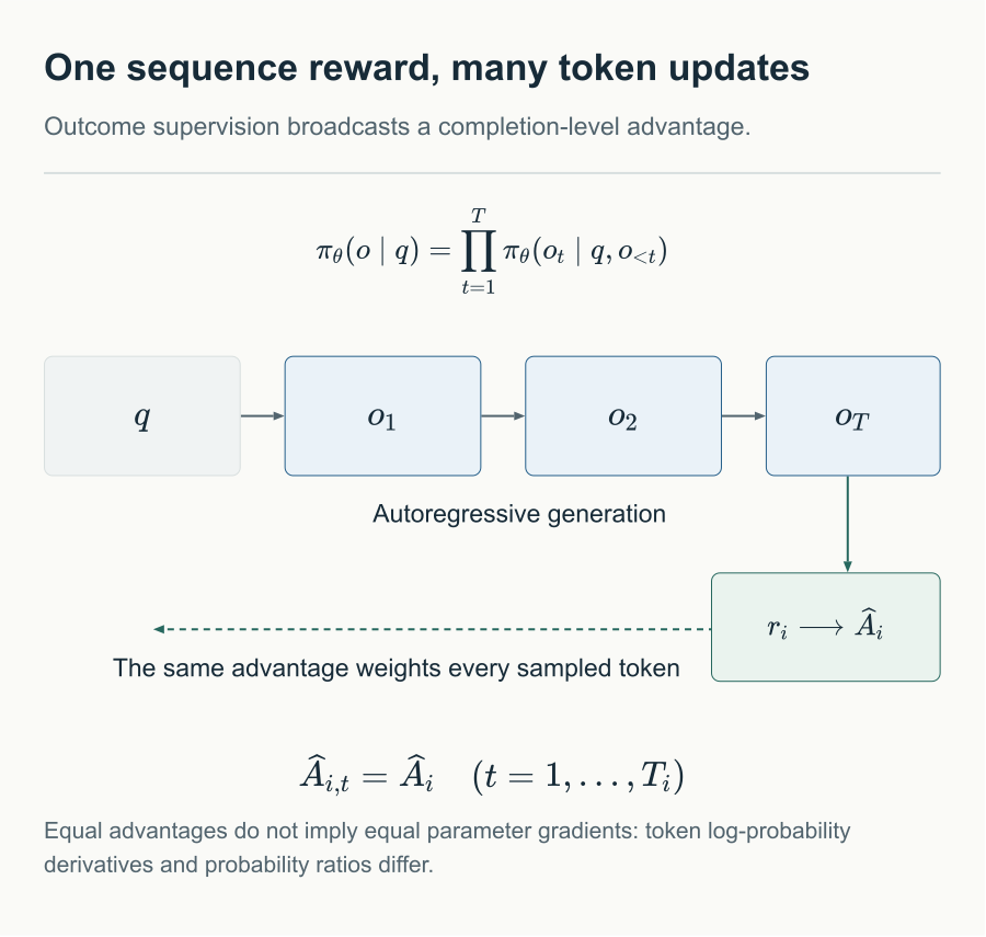
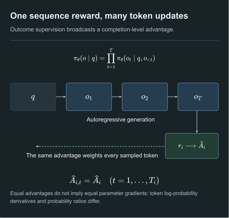
Outcome supervision shares one advantage across a completion; token gradients can still differ.
This is the concrete shape of everything the abstract sections built: tokens are actions, the growing context is the state, the completion is the trajectory, and the one reward at the end is spread back across the tokens that produced it.
One Gradient, Many Methods
There is a vantage point from which GRPO, PPO, and the method of the next chapter are visibly the same construction, and reaching it is the cleanest way to set up what comes next. Write the gradient of every method in this family in one form:
Every method here is a weighted maximum-likelihood objective on generated sequences: it pushes up the log-probability of tokens, and the only thing that differs between methods is the weight on each token and where the data comes from.
| Method | Data source | Gradient coefficient |
|---|---|---|
| Supervised fine-tuning | fixed demonstrations | |
| Rejection sampling | model's correct samples | |
| PPO | on-policy samples | (critic advantage) |
| GRPO | on-policy groups | (group advantage + KL) |
| DPO | preference pairs | a preference weight (next chapter) |
Seen this way, "reinforcement learning fine-tuning" is reweighted imitation. Supervised fine-tuning imitates every demonstration equally; rejection sampling imitates only the correct samples; PPO and GRPO imitate on-policy samples weighted by how much better than average they were. The reinforcement-learning machinery, the sampling loop, the reward model, the advantage, the clip, all of it, exists to compute the weight for each token.
If the machinery only exists to compute a weight, the natural question is whether the weight can be computed without the machinery. For preference data the answer is yes. The next chapter takes the KL-regularized objective introduced above, solves it exactly, and finds that the optimal policy's own log-probabilities encode the reward, so the weight can be written in closed form from a pair of completions with no sampling loop, no reward model, and no advantage. GRPO removed the critic; Direct Preference Optimization removes the loop.
Further Reading
This chapter assumed the clipped surrogate, the probability ratio, and the analysis of what clipping guarantees from Proximal Policy Optimization, and the baseline theorem and advantage from Policy Gradient.
The KL-regularized objective built in the middle of the chapter is the shared starting point of the next one, where it is not optimized by sampling but solved in closed form. The Bradley-Terry reward model defined in the application section is the object that chapter shows can be bypassed: its per-prompt shift ambiguity, noted above as a technicality, is exactly what cancels.
References
- Shao, Z., Wang, P., Zhu, Q., Xu, R., Song, J., et al. (2024). DeepSeekMath: Pushing the Limits of Mathematical Reasoning in Open Language Models. arXiv:2402.03300. Introduces GRPO (§4) and the unified-paradigm view (§5.2.1).
- Ouyang, L., Wu, J., Jiang, X., et al. (2022). Training Language Models to Follow Instructions with Human Feedback. arXiv:2203.02155. The RLHF pipeline and the per-token KL-in-reward formulation.
- Schulman, J. (2020). Approximating KL Divergence. joschu.net/blog/kl-approx.html. The estimator used for the divergence term.
- Bradley, R. A., & Terry, M. E. (1952). Rank Analysis of Incomplete Block Designs: I. The Method of Paired Comparisons. Biometrika, 39(3/4), 324-345.
Comments