Mathematical Setting and What Can Be Identified
Let be a conditioning input and let be a candidate output. Conditional on , the policy and reference policy are distributions over outputs, denoted and . We write the argument first for a discrete output space. For continuous outputs, replace sums by integrals and probabilities by densities with respect to a common base measure.
Fix a global regularization coefficient . On the policy support allowed for each , require , and require the partition function defined below to be finite. The support condition matters: KL regularization cannot place optimal probability mass where the reference policy assigns exactly zero probability. DPO therefore cannot discover outputs outside the reference policy’s support.
Preference data are not deterministic truth labels. We observe noisy paired comparisons , where records whether the annotator prefers . It is conventional to reorder each observation into a winner and a loser , absorbing the label into the order. The logistic loss below is the conditional maximum likelihood of this stochastic comparison model, not a claim that every preference is an inviolable fact.
A General Preference-Learning Paradigm
Group Relative Policy Optimization ended with an objective: improve task reward without drifting too far from a frozen reference policy.
GRPO approximately optimizes it with a reinforcement-learning loop: sample from the current policy, score outputs, estimate advantages, then update the policy. When rewards come from paired preferences, the usual route first fits a reward model to those pairs. That route has two learning stages: learn , then optimize by reinforcement learning.
The question here is narrower. If the preference pairs are already available, can we optimize the policy directly, without explicitly fitting a reward model and without drawing outputs from the policy during training?
Direct Preference Optimization (DPO) answers yes [1][1] R. Rafailov, A. Sharma, E. Mitchell, S. Ermon, C. D. Manning, and C. Finn, “Direct Preference Optimization: Your Language Model Is Secretly a Reward Model,” Advances in Neural Information Processing Systems, vol. 36, 2023. https://proceedings.neurips.cc/paper_files/paper/2023/hash/a85b405ed65c6477a4fe8302b5e06ce7-Abstract-Conference.html. It does not delete reinforcement learning by fiat. Instead, it solves the KL-regularized problem above and observes that preference data are exactly sufficient to eliminate the reward from that solution.
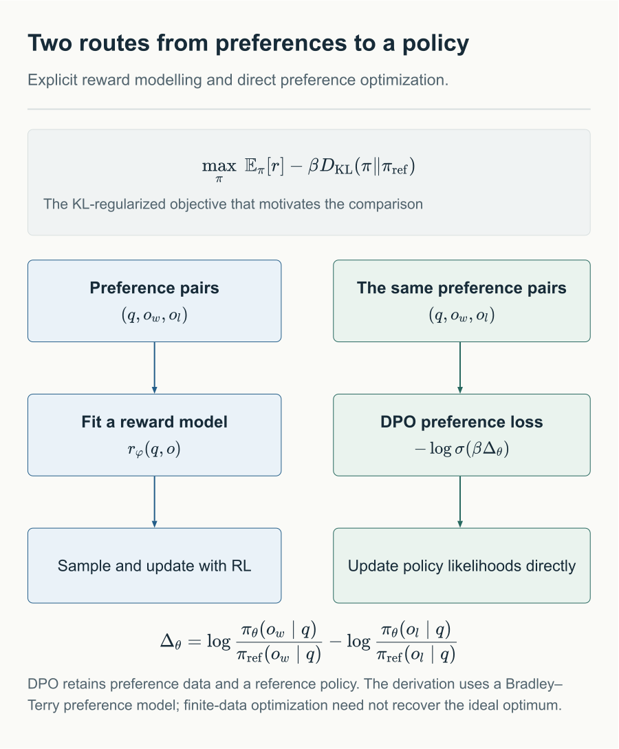
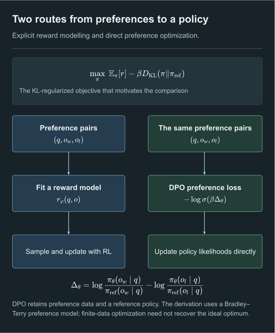
DPO uses preference pairs and a reference policy to update policy likelihoods directly, avoiding a separately trained reward model in this route.
Both routes can begin with the same preference dataset. Their difference is not whether preference is assumed. It is whether preference is first compressed into an explicit reward and then used for online policy optimization.
Read as a general conditioning input and as a candidate output comparable under that input. Then may be any conditional probability distribution defined by a neural network: a text generator, an action policy, a candidate-structure generator, or another model that can assign a probability or density to a candidate output. DPO is not specific to language models.
It is not, however, a loss that can be applied unchanged to every deterministic network. The derivation compares , so the model must define a computable conditional probability or density. A network that only emits a point estimate needs a separate probabilistic model or a different preference objective.
First Fix One Conditioning Input
The derivation is clearest before mixing conditioning inputs together. Fix , abbreviate the output-space policy as , the reference policy as , and the reward as . We solve
subject to and whenever . Here controls the trade-off between reward and staying near the reference policy.
This is not yet a policy-gradient problem. For the moment is any distribution on the output space, so the problem is ordinary constrained optimization.
For fixed , if
then the objective is strictly concave on the reference support and has the unique optimum
where normalizes the probabilities to sum to one.
Introduce a Lagrange multiplier for normalization. In the interior of the reference support, the derivative of the Lagrangian with respect to each is
Rearranging and exponentiating gives
The final factor does not depend on . Normalization makes it , yielding the stated form.
This is more than a stationary point. The reward term is linear in , while is strictly concave on the reference support, so the stationary point is the unique global maximum.
The equation says more than “higher reward means more probability.” Reward does not create a distribution from nothing. It exponentially tilts probability that the reference policy already assigns. For any ,
Thus a very small reference probability can still be reversed by a finite reward difference. The result depends jointly on the reference probability ratio, reward difference, and . The strict boundary is only the support result: finite reward cannot bring an output with exactly zero reference probability into the optimum.
The Reward Is Hidden in a Policy Ratio
Taking logs of the optimal policy and rearranging yields
This is DPO’s central equation. It associates an optimal policy with a reward function: knowing how changes log probability relative to recovers a compatible reward, up to the conditioning-input-only constant .
For a fixed , adding the same constant to every output’s reward does not change which policy is optimal. This freedom is exactly the term. It is not a hole in the derivation. Paired preference data can identify reward differences only.
No preference data have been used yet. The next step explains why one winner-loser pair is enough to remove this unknown constant.
Preferences See Differences Only
For the same , let be the preferred output and the alternative. DPO uses the Bradley-Terry random-utility model: conditional on the two outputs, preference probability depends only on their latent reward difference,
where [2][2] R. A. Bradley and M. E. Terry, “Rank Analysis of Incomplete Block Designs: I. The Method of Paired Comparisons,” Biometrika, vol. 39, no. 3/4, pp. 324–345, 1952. https://doi.org/10.1093/biomet/39.3-4.324.
Substitute the optimal-policy reward expression for and . The terms for the same conditioning input cancel:
This is why DPO works. A preference label does not require the absolute reward of either output. It requires only which is preferred. The normalization constant in the KL-regularized optimum is also a per-input constant, so it disappears within the same pair. If preferences cannot be represented by a scalar reward difference, or do not obey the Bradley-Terry link, this loss is a model-misspecified approximation. The algebra above does not by itself prove it correct.
From an Optimal Policy to a Trainable Model
In training we do not know ; we have a parameterized model family and a finite dataset. We therefore replace the in the Bradley-Terry model with and maximize the conditional likelihood of observed preference pairs. This is a statistical modeling and projection step, not a pointwise identity that turns every statement about the true into a statement about arbitrary . Only with sufficient model capacity, a correct preference model, infinite data, and population-optimal training would the corresponding preference probabilities be recovered.
Define the log-ratio difference
The DPO loss is then
It is binary negative log likelihood. The model should increase the winner’s probability relative to the reference policy by more than it increases the loser’s. In practice a minibatch mean estimates this expectation. There is no explicit and no inner loop that generates rollouts from the current policy.
What One Update Actually Pushes
Write the DPO objective as maximizing . For one preference pair,
It has three parts:
- the first raises the probability of the winner;
- the second lowers the probability of the loser;
- determines how much learning signal remains. It approaches zero when the model already strongly favors the winner, and is larger when the preference is not yet learned.
More generally, this is a weighted conditional log-likelihood gradient. Its weight no longer comes from online sampling, reward scoring, and advantage estimation. It comes directly from the classification error of an offline preference pair. If an output is composed of local decisions, the particular model further factorizes into the relevant local probabilities.
Beta Is Still the KL Knob
The in the loss is not merely a temperature in front of a logistic function. It comes from the original KL-regularized objective,
In the sense of a correctly specified population model trained to convergence, a larger means a stronger reference-policy constraint: the exponential tilt in is weaker. The same parameter also scales the relative log-probability difference in DPO, changing gradient scale during finite training. A larger or smaller gradient in one run must not be equated directly with a final policy that necessarily moves farther or less far.
Removing reduces DPO to ordinary preference classification that merely tries to make more probable than . The reference model turns “raise the winner” into a change relative to the original model and preserves the original KL-regularized objective in the loss.
What DPO Removes, and What It Does Not
| Component | Reward-model-plus-RL route | DPO |
|---|---|---|
| Paired preference data | Trains the reward model | Trains the policy directly |
| Explicit reward model | Required | Not required |
| Policy sampling during training | Required | Not required |
| Critic and advantage | Depends on the RL algorithm | Not required |
| Reference policy | KL anchor | Still required |
| Preference assumption | Bradley-Terry or related model | Still required |
DPO removes explicit reward modeling and the online reinforcement-learning loop, not preference learning itself. It still needs high-quality preference pairs and still assumes those preferences can be explained by an implicit reward relative to the reference policy.
This also gives its boundary. DPO optimizes a fixed preference dataset. Unlike online RL, it cannot actively explore outputs that the current policy has not produced; if the dataset does not cover an error or a better candidate, the loss will not discover it from nothing. Its simplicity comes from limiting the learning signal to existing paired comparisons, not from receiving a more complete form of feedback for free.
Application: DPO for Language Models
A language model is one instance of the general paradigm. Here the conditioning input is a prompt, the candidate output is a complete completion, and is the model’s conditional probability of that completion.
Its special feature is that a completion is a sequence of tokens, so its log probability factorizes exactly as
Substituting this into the DPO loss gives one preference label for a pair of full completions, but distributes gradient across the conditional probability of every token. This resembles supervised fine-tuning in form. The difference is that supervised fine-tuning only raises the probability of a demonstration, whereas DPO raises the winner, lowers the loser, and measures both movements relative to the reference model.
The original DPO paper validates the method primarily on language-model preference data [1][1] R. Rafailov, A. Sharma, E. Mitchell, S. Ermon, C. D. Manning, and C. Finn, “Direct Preference Optimization: Your Language Model Is Secretly a Reward Model,” Advances in Neural Information Processing Systems, vol. 36, 2023. https://proceedings.neurips.cc/paper_files/paper/2023/hash/a85b405ed65c6477a4fe8302b5e06ce7-Abstract-Conference.html, which is why that setting is encountered first. The derivation itself uses only conditional distributions, a reference policy, KL regularization, and a paired-preference model. In another probabilistic neural model, , , and the probability factorization change. The core DPO logic does not.
From GRPO to DPO
GRPO and DPO are not unrelated tricks. GRPO starts from the KL-regularized objective and uses sampling plus advantage estimation to optimize reward. DPO starts from the same objective, first solves for the optimal policy, then uses preference pairs to eliminate reward and the normalization constant. The former suits settings that can score new outputs; the latter suits settings that already contain offline preference pairs.
Their real dividing line is not whether either one is “alignment.” It is where the learning signal lives: GRPO receives a scalar evaluation of current outputs, while DPO receives a fixed winner-loser comparison. Both try to improve preference agreement while retaining the prior behavior supplied by the reference model.
Further Reading
The original paper presents DPO as direct optimization of a KL-constrained reward-maximization problem and validates it on language-model preference data [1][1] R. Rafailov, A. Sharma, E. Mitchell, S. Ermon, C. D. Manning, and C. Finn, “Direct Preference Optimization: Your Language Model Is Secretly a Reward Model,” Advances in Neural Information Processing Systems, vol. 36, 2023. https://proceedings.neurips.cc/paper_files/paper/2023/hash/a85b405ed65c6477a4fe8302b5e06ce7-Abstract-Conference.html. This chapter gives the general conditional-distribution derivation first, then treats language models as one application. Extending DPO to token-level MDPs, online preference learning, or other divergences requires additional assumptions; it does not follow automatically from this page.
References
- [1] R. Rafailov, A. Sharma, E. Mitchell, S. Ermon, C. D. Manning, and C. Finn, “Direct Preference Optimization: Your Language Model Is Secretly a Reward Model,” Advances in Neural Information Processing Systems, vol. 36, 2023. https://proceedings.neurips.cc/paper_files/paper/2023/hash/a85b405ed65c6477a4fe8302b5e06ce7-Abstract-Conference.html a b c
- [2] R. A. Bradley and M. E. Terry, “Rank Analysis of Incomplete Block Designs: I. The Method of Paired Comparisons,” Biometrika, vol. 39, no. 3/4, pp. 324–345, 1952. https://doi.org/10.1093/biomet/39.3-4.324 ↩
Comments