Number Systems, Algorithms, and Recursion

The earlier chapters separate three questions: what belongs to a set, how functions pair elements, and how a sequence assigns values to indices. Here those ideas meet arithmetic and computation. We first compare the standard number systems, then study the integer operations used by algorithms, and finally prove that iterative and recursive procedures do what they claim.

The prerequisites are Naive Set Theory, Functions and Mappings, and Sequences and Series. Throughout, $\mathbb N=\{0,1,2,\ldots\}$; positive integers are written $\mathbb Z_{>0}$. The treatments of infinite sets, recursive data, and invariants in Mathematics for Computer Science provide further practice [1][1] E. Lehman, F. T. Leighton, and A. R. Meyer, Mathematics for Computer Science. MIT OpenCourseWare, 2015. Revised May 18, 2015; infinite sets, recursive data, and invariants. https://ocw.mit.edu/courses/6-042j-mathematics-for-computer-science-spring-2015/mit6_042js15_textbook.pdf.

Number systems extend the available operations

The familiar inclusions are

$$\mathbb N\subsetneq\mathbb Z\subsetneq\mathbb Q \subsetneq\mathbb R\subsetneq\mathbb C.$$

Under these standard identifications, moving right retains the earlier numbers while permitting new solutions or limits.

System	What it contains	What the extension provides
$\mathbb N$	$0,1,2,\ldots$	Counting and induction
$\mathbb Z$	Integers, positive, negative, and zero	Subtraction always stays in the system
$\mathbb Q$	Ratios $p/q$, with integers $p,q$ and $q\ne0$	Division by any nonzero element
$\mathbb R$	Rational and irrational real numbers	A complete ordered field
$\mathbb C$	Numbers $a+bi$, with $a,b\in\mathbb R$ and $i^2=-1$	A solution of $x^2=-1$ and a broader algebraic setting

The first steps can be motivated by equations: $x+3=1$ has no solution in $\mathbb N$, and $2x=1$ has no solution in $\mathbb Z$. Passing from $\mathbb Q$ to $\mathbb R$ also addresses limiting processes, not just one missing root. Complex numbers are developed in their own chapter.

A rational number has many fractional representations. For nonzero denominators,

$$\frac pq=\frac rs\quad\Longleftrightarrow\quad ps=rq.$$

The fractions $1/2$ and $2/4$ therefore represent one number, not two elements of $\mathbb Q$. A formal construction treats equivalent integer pairs as the same rational number; this is an application of equivalence classes.

The irrational numbers form $\mathbb R\setminus\mathbb Q$. They are not another nested field: $\sqrt2$ and $-\sqrt2$ are irrational, but their sum is rational. Prime numbers likewise form a special subset of $\mathbb N$, rather than a new number system in the inclusion chain. A prime is an integer greater than $1$ whose only positive divisors are $1$ and itself; in particular, $1$ is not prime.

Decimal representations are not the numbers themselves

A rational number has a terminating or eventually periodic decimal expansion. In long division by a positive denominator $q$, there are only $q$ possible remainders. A zero remainder ends the expansion; otherwise a remainder repeats and the subsequent digits repeat. Conversely, an eventually repeating tail is a geometric series, so it represents a rational number.

For instance, $1/3=0.\overline3$. Decimal expansions can also have two representations of the same value: $0.999\ldots=1$. Infinite nonperiodic decimals represent irrational numbers, but merely seeing a long finite prefix does not establish nonperiodicity. A real number can be approximated by rational decimal truncations; this is a property of the real system, not a self-contained construction of it before limits have been defined.

Cardinality: Cantor’s diagonal argument

The rationals are dense: between any two distinct rationals there is another rational. Yet they can still be listed. To prove that the reals are uncountable, we need a different obstruction: every proposed list misses a real number, regardless of how cleverly it is arranged.

TheoremThe interval (0,1) is uncountable

There is no sequence $x_1,x_2,\ldots$ whose entries include every real number in $(0,1)$.

The indices here start at $1$ to match the decimal places. Starting at $0$ instead would not affect countability. Repetitions in the proposed list are allowed: even a list with repetitions cannot cover the interval.

Step 1: suppose a complete list exists

Proof

Assume that all the reals in $(0,1)$ appear in a sequence. For each entry, choose the decimal expansion that is not eventually all nines. For example, use $0.5000\ldots$ rather than $0.4999\ldots$.

Write

$$x_k=0.d_{k1}d_{k2}d_{k3}\ldots.$$

The first subscript specifies the row; the second specifies a digit position. Thus $d_{kn}$ is the $n$th decimal digit of the $k$th number. A finite table can display only finitely many rows and columns, but the assumed list and all its decimal expansions continue indefinitely.

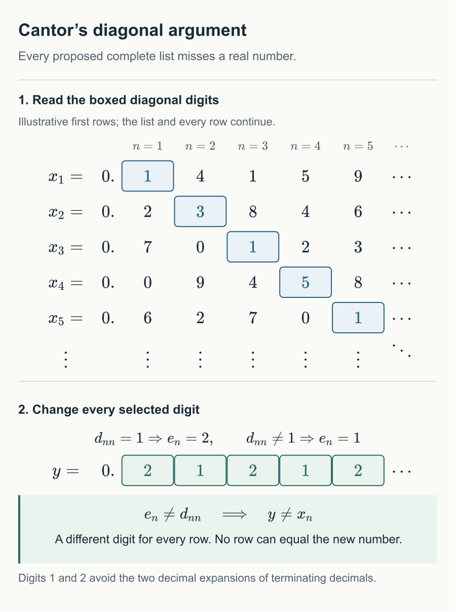
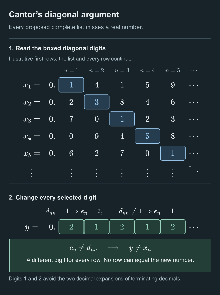
The diagonal digits shown are $1,3,1,5,1$; the construction changes them to $2,1,2,1,2$. Only the first five positions are displayed: the rule defines every subsequent digit as well.

Step 2: change the diagonal, one digit per row

Read $d_{11},d_{22},d_{33},\ldots$: the first digit of the first number, the second digit of the second number, and so on. Define

$$e_n= \begin{cases} 1,&d_{nn}\ne1,\\ 2,&d_{nn}=1. \end{cases}$$

In either case, $e_n\ne d_{nn}$. The essential choice is the pairing of row $n$ with position $n$: we reserve a specific position at which to defeat each row.

Step 3: the new digits define a real number

Set $y=0.e_1e_2e_3\ldots$. More explicitly,

$$y=\sum_{n=1}^{\infty}\frac{e_n}{10^n}.$$

Because each digit is $1$ or $2$, the partial sums are increasing and bounded. They define a real number, with

$$\frac19\le y\le\frac29.$$

These bounds follow from the geometric series with all digits equal to $1$ or all equal to $2$. In particular, $y\in(0,1)$, so it belongs to the set that the list supposedly covers.

Step 4: no row can equal the new number

Choose any row $k$. At position $k$, the number in that row has digit $d_{kk}$, while $y$ has digit $e_k$. By construction,

$$e_k\ne d_{kk}\quad\Longrightarrow\quad y\ne x_k.$$

The implication uses our decimal convention: all listed expansions avoid eventual nines, and the expansion of $y$, containing only ones and twos, has no terminating-decimal ambiguity. A full explanation is given below.

Since $k$ was arbitrary, $y$ differs from every number in the list. But $y$ is in $(0,1)$ and should therefore occur in a complete list. This contradiction proves that no such list exists.

Why the decimal convention matters

A difference between two digit strings does not always mean a difference between the numbers they represent. For example,

$$0.5000\ldots=0.4999\ldots.$$

Changing diagonal digits to $0$ or $9$ without handling this issue could leave a gap in the proof. Our construction uses only $1$ and $2$, so its expansion is neither eventually zero nor eventually nine. The proposed list also uses the convention excluding eventual nines.

Why these are the only ambiguous decimal expansions

Suppose two decimal strings first differ at position $N$, with $a_N<b_N$. The advantage of the larger digit is at least $10^{-N}$. The entire tail can compensate by at most

$$\sum_{n>N}\frac9{10^n}=10^{-N}.$$

Equality between the represented numbers is therefore possible only if $b_N=a_N+1$, the smaller-digit string has nothing but nines after position $N$, and the larger-digit string has nothing but zeros after that position. Any smaller tail compensation leaves a strict difference.

This explains both $0.4999\ldots=0.5000\ldots$ and why excluding eventual nines gives a unique expansion. It also shows directly that a string containing only ones and twos cannot participate in such an ambiguity.

What the argument does and does not say

The constructed number depends on the proposed list. The conclusion is “for every list, there exists a missing number,” not that one fixed number is missing from every list. If a new list includes the previous missing number, apply the same construction to that new list: it produces another missing number. An infinite list also has no final row after which a number can simply be appended.

Nor does the construction prove that its new number is irrational. Depending on the diagonal, its digits might repeat. What matters is that it is a real number outside the proposed list. Applying a similar digit-changing rule to a list of rationals does not contradict their countability, because the constructed real number need not be rational.

Since $(0,1)\subseteq\mathbb R$, the real numbers are uncountable too. The irrationals are also uncountable: if they were countable, interleaving their list with a list of the rationals would make all reals countable, contradicting the result just proved.

The same “disagree with row $n$ at position $n$” pattern appears for infinite binary sequences in Sequences and Common Sequences and for subsets of the natural numbers in Naive Set Theory. The objects change; the diagonal construction serves the same purpose.

Countability, numerical order, and available operations must be assessed separately. Adding negative numbers or rational fractions does not change the countably infinite cardinality of the natural numbers; extending to all real numbers does.

Fields, order, and completeness

A field makes arithmetic reversible where permitted

DefinitionField

A field $F$ has addition and multiplication mapping $F\times F$ into $F$, and distinct elements $0,1$. Addition is associative and commutative, has identity $0$, and gives every element an additive inverse. Multiplication is associative and commutative, has identity $1$, and gives every nonzero element a multiplicative inverse. Multiplication distributes over addition.

Subtraction means adding an additive inverse; division by a nonzero element means multiplying by its inverse. These axioms hold in $\mathbb Q$, $\mathbb R$, and $\mathbb C$, but not in $\mathbb Z$, where $2$ has no multiplicative inverse, or in $\mathbb N$, where $1$ has no additive inverse.

ProofWhy zero has no inverse and cancellation needs a condition

Distributivity gives

$$x\cdot0=x(0+0)=x\cdot0+x\cdot0.$$

Subtracting $x\cdot0$ yields $x\cdot0=0$. Therefore $0u$ cannot equal $1$.

If $xz=yz$ and $z\ne0$, multiplying by $z^{-1}$ gives $x=y$. If $z=0$, the equality holds for all $x,y$ and provides no such conclusion. Likewise, if $xy=0$ and $x\ne0$, multiplying by $x^{-1}$ gives $y=0$: a field has no nonzero zero divisors.

Order must be compatible with arithmetic

DefinitionOrdered field

An ordered field is a field equipped with a total order $\le$. The order is reflexive, antisymmetric, transitive, and compares every two elements. It satisfies

$$x\le y\quad\Longrightarrow\quad x+z\le y+z,$$

and multiplying a strict inequality by a positive element preserves it:

$$x<y,\quad z>0\quad\Longrightarrow\quad xz<yz.$$

Here antisymmetry uses $x\le y$ and $y\le x$ to conclude $x=y$. For the strict order, exactly one of $x<y$, $x=y$, and $y<x$ holds. Omitting the equality case would fail already when $x=y$.

Multiplying by a negative number reverses inequalities. Every square is nonnegative: if $x\ge0$, multiply nonnegative factors; if $x<0$, use $x^2=(-x)^2$ with $-x>0$. In particular $1>0$, and $0<x<y$ implies $0<1/y<1/x$ by multiplying $x<y$ by the positive number $1/(xy)$.

The usual orders make $\mathbb Q$ and $\mathbb R$ ordered fields. No order can make $\mathbb C$ an ordered field, because $i^2=-1$ would be a nonnegative square, contradicting $1>0$. The issue is compatibility with field operations, not whether complex numbers can be ordered by some other rule.

Completeness fills an order-theoretic gap

An upper bound $u$ for a subset $S$ satisfies $s\le u$ for all $s\in S$. A supremum, or least upper bound, is an upper bound no larger than any other upper bound. A maximum must belong to $S$; a supremum need not. For example, $(0,1)$ has supremum $1$ and no maximum.

DefinitionCompleteness of an ordered field

An ordered field is complete if every nonempty subset that is bounded above has a supremum in that field. The real numbers form a complete ordered field.

The qualifier “in that field” matters. The rational set

$$S=\{q\in\mathbb Q:q\ge0,\ q^2<2\}$$

has supremum $\sqrt2$ in $\mathbb R$, but no supremum in $\mathbb Q$. Rational numbers approach $\sqrt2$ from below, and every rational upper bound can be decreased while remaining above $\sqrt2$. Irrationality of $\sqrt2$ was proved in Indirect Proof. Density of rational numbers in the real line explains these approximations; one proof is an exercise below. Having a number between two others is weaker than having every required supremum. Further development of complete ordered fields is given in Lebl’s Basic Analysis [2][2] J. Lebl, Basic Analysis I: Introduction to Real Analysis, Volume I. . Online edition; Sections 1.1--1.2 on ordered fields and completeness; accessed September 6, 2026. https://www.jirka.org/ra/html/.

Completeness also implies that natural numbers are unbounded above in $\mathbb R$. Otherwise, if $s=\sup\mathbb N$, the smaller number $s-1$ would not be an upper bound, so some $n\in\mathbb N$ would satisfy $n>s-1$. Then $n+1>s$, contradicting the bound. This Archimedean property ensures integers can be found beyond any fixed real threshold, as needed for floor and ceiling.

Floor, ceiling, and Euclidean remainders

DefinitionFloor and ceiling

For real $x$, the floor $\lfloor x\rfloor$ is the greatest integer at most $x$, and the ceiling $\lceil x\rceil$ is the least integer at least $x$. Their defining bounds are

$$\lfloor x\rfloor\le x<\lfloor x\rfloor+1,$$$$\lceil x\rceil-1<x\le\lceil x\rceil.$$

The Archimedean property and the well-ordering of the nonnegative integers ensure these integers exist. Floor rounds downward, not toward zero: $\lfloor-2.3\rfloor=-3$, whereas $\lceil-2.3\rceil=-2$. At an integer $k$, both equal $k$.

For every integer $k$, floor is constant at $k$ on $[k,k+1)$, while ceiling is constant at $k$ on $(k-1,k]$. These half-open intervals specify the endpoint values precisely.

ProofNegation exchanges floor and ceiling

Put $m=\lceil x\rceil$. Its bounds give $m-1<x\le m$. Negating reverses the inequalities:

$$-m\le-x<-m+1.$$

Thus $\lfloor-x\rfloor=-m=-\lceil x\rceil$. Replacing $x$ by $-x$ also gives $\lceil-x\rceil=-\lfloor x\rceil$.

A positive divisor fixes the remainder convention

Let $a\in\mathbb Z$ and $m\in\mathbb Z_{>0}$. Set

$$q=\left\lfloor\frac am\right\rfloor, \qquad r=a-mq.$$

The floor bounds imply $mq\le a<m(q+1)$, hence

$$a=mq+r,\qquad 0\le r<m.$$

This proves existence of the Euclidean quotient and remainder. For uniqueness, two such expressions would give $m(q-q')=r'-r$. The right side lies strictly between $-m$ and $m$, whose only integer multiple of $m$ is zero. Therefore $q=q'$ and $r=r'$.

We write $a\bmod m=r$. For example, $-17=5(-4)+3$, so $-17\bmod5=3$. Divisibility means $m\mid a$ if $a=mk$ for some integer $k$; for a positive $m$, this is equivalent to a zero remainder. Programming-language operators and conventions for negative divisors must be checked separately; all remainder operations below use positive divisors.

Algorithms need a contract and a correctness argument

A procedure consists of precise, executable steps. To claim that it solves a problem on a specified domain, state valid inputs and required outputs, prove it terminates on every valid input, and prove the returned result meets that requirement. Correctness is not established merely because the arithmetic problem has a solution.

Pseudocode describes these steps without committing to a programming language. The symbol $\gets$ means assignment; an equality in a proof states a mathematical relation. We use exact arithmetic here, so machine overflow is outside this model.

Halving and doubling multiplication

Given $M\in\mathbb Z$ and $N\in\mathbb N$, the following algorithm returns $MN$. Only the second input must be nonnegative; zero is included.

Algorithm 1 Halving and Doubling Multiplication

Require: $M \in \mathbb{Z}$, $N \in \mathbb{N}$

Ensure: the product $MN$

1:$A \gets M$, $B \gets N$, $p \gets 0$

2:while $B > 0$ do

3:if $B \bmod 2 = 1$ then

4:$p \gets p+A$

5:end if

6:$A \gets 2A$

7:$B \gets \lfloor B/2 \rfloor$

8:end while

9:return $p$

For $M=73,N=41$, the loop visits the following values before updating them:

$A$	$B$	Contribution to $p$
$73$	$41$	$73$
$146$	$20$	$0$
$292$	$10$	$0$
$584$	$5$	$584$
$1168$	$2$	$0$
$2336$	$1$	$2336$

The sum is $73+584+2336=2993=73\cdot41$.

ProofInvariant and termination

At the start of every iteration, the invariant is $p+AB=MN$. It holds initially. Write the current $B=2q+r$, where $r\in\{0,1\}$. One full iteration changes the state to $p'=p+rA$, $A'=2A$, $B'=q$, giving

$$\begin{aligned} p'+A'B'&=p+rA+2Aq\\ &=p+A(2q+r)\\ &=p+AB. \end{aligned}$$

Thus the invariant is preserved in both parity cases. While $B>0$, its new value $\lfloor B/2\rfloor$ is a strictly smaller nonnegative integer. The loop therefore terminates. At termination $B=0$, and the invariant yields $p=MN$. If $N=0$, the loop is skipped and the result is already correct.

Complexity depends on the input size and cost model

For $N>0$, after $k$ completed iterations, while that state exists,

$$B_k=\left\lfloor\frac{N}{2^k}\right\rfloor.$$

Repeated integer halving gives this expression; it follows by dividing $N$ into a multiple of $2^k$ and a remainder. If $2^{L-1}\le N<2^L$, then $B_{L-1}=1$ and $B_L=0$. Hence the exact iteration count is

$$L=\lfloor\log_2N\rfloor+1.$$

This counts the iteration starting with $B=1$. For $N=0$, there are zero iterations and no logarithm is used. The value $L$ is also the binary length of a positive $N$, so logarithmic dependence on the numerical value is linear dependence on that input’s bit length.

DefinitionBig-O and a tight bound

For eventually nonnegative functions $T,f$ on the natural numbers, write $T(n)=O(f(n))$ if there exist constants $c>0$ and $n_0$ such that

$$0\le T(n)\le c f(n)\qquad(n\ge n_0).$$

Write $T(n)=\Theta(f(n))$ when both upper and lower bounds by positive constant multiples of $f(n)$ hold eventually.

Big-O is an asymptotic upper bound on a function, not a statement that an algorithm has been measured, nor a synonym for worst-case analysis. One may bound a worst-case, average-case, or other specified cost function. Common growth rates include $1$, $\log n$, $n$, $n\log n$, $n^2$, and $2^n$.

If each exact integer operation is charged one unit, multiplication above uses $\Theta(L)$ loop work for $N>0$ and a constant number of integer registers. That does not mean constant memory in bits: those registers store larger integers as inputs grow. With ordinary binary representations and schoolbook operations, an upper bound is $O(L(M_b+L))$ bit operations and $O(M_b+L)$ working bits, where $M_b$ is the bit length of $|M|$, taking at least one bit for zero. This bound charges up to $O(M_b+L)$ for each iteration. A sharper implementation analysis may improve it, but must still state its model.

Recursion defines objects by smaller objects

A recursive definition needs starting cases, construction rules, and a reason the recursive dependencies cannot descend forever. For instance,

$$0!=1,\qquad (n+1)!=(n+1)n!$$

defines a unique value for each $n\in\mathbb N$: reaching the next value uses one already defined. A recursive evaluation of $n!$ reduces the nonnegative argument until it reaches zero. A formula referring to itself does not by itself guarantee existence, uniqueness, or termination.

Finite full binary trees

Define trees by exactly these rules: $\operatorname{Leaf}$ is a tree, and if $L,R$ are trees, then $\operatorname{Node}(L,R)$ is a tree. Nothing else is a tree. Here constructors are distinct and their arguments are ordered, so every non-leaf has unique left and right subtrees. These are finite full binary trees, built using finitely many constructor applications; every internal node has exactly two children.

Define the number of leaves $\ell$ and internal nodes $i$ recursively:

$$\ell(\operatorname{Leaf})=1,\qquad i(\operatorname{Leaf})=0,$$ $$\ell(\operatorname{Node}(L,R))=\ell(L)+\ell(R),$$ $$i(\operatorname{Node}(L,R))=1+i(L)+i(R).$$

This gives a recursive algorithm for counting leaves:

Algorithm 2 Count Leaves

Require: a finite full binary tree $T$

Ensure: the number of leaves in $T$

1:if $T=\operatorname{Leaf}$ then

2:return $1$

3:else

4:let $T=\operatorname{Node}(L,R)$

5:$a \gets$ CountLeaves($L$)

6:$b \gets$ CountLeaves($R$)

7:return $a+b$

8:end if

Each call uses a proper subtree with fewer nodes, so recursion terminates on the specified finite inputs. This justification would not automatically apply to infinite trees.

Structural induction follows the construction rules

To prove a property for every tree, prove it for $\operatorname{Leaf}$, then assume it for arbitrary $L,R$ and prove it for $\operatorname{Node}(L,R)$. These cases cover every permitted finite construction. This is structural induction; induction on natural numbers is the corresponding pattern for zero and successor.

ProofLeaves are one more than internal nodes

For a leaf, $\ell=1=i+1$. Suppose $\ell(L)=i(L)+1$ and $\ell(R)=i(R)+1$, and put $T=\operatorname{Node}(L,R)$. Then

$$\begin{aligned} \ell(T)&=\ell(L)+\ell(R)\\ &=i(L)+i(R)+2\\ &=i(T)+1. \end{aligned}$$

Thus every finite full binary tree has exactly one more leaf than internal nodes. The hypotheses concern both immediate subtrees, rather than an unspecified “previous tree.”

Exercises

ExerciseCountable size, supremum, and maximum

For $S=\{1-1/n:n\in\mathbb Z_{>0}\}$, determine its cardinality, supremum, and whether it has a maximum.

Show solution

Solution

The listed values are strictly increasing, giving a bijection from positive integers onto $S$, so $S$ is countably infinite. Every value is less than $1$. If $u<1$, choose an integer $n>1/(1-u)$ using the Archimedean property; then $1-1/n>u$. Thus no number below $1$ is an upper bound, and $\sup S=1$. It is not a maximum because $1\notin S$; also the next listed value always exceeds the current one.

ExerciseFind a rational between two reals

Let $a<b$ be real. Use the Archimedean property and floor to find integers $p$ and $n>0$ such that $a<p/n<b$.

Show solution

Solution

Choose a positive integer $n$ with $n(b-a)>1$, then put $p=\lfloor na\rfloor+1$. The floor bounds give

$$na<p\le na+1<nb.$$

Dividing by positive $n$ proves the claim. This establishes density in the real line without implying uncountability of $\mathbb Q$.

ExerciseTranslate floor comparisons into real inequalities

For integer $m$, characterize each condition: $\lfloor x\rfloor<m$, $m\le\lfloor x\rfloor$, $\lfloor x\rfloor\le m$, $m<\lfloor x\rfloor$, $\lfloor x\rfloor=m$, and $\lceil x\rceil=m$.

Show solution

Solution

Their equivalent conditions, in the same order, are

$$\begin{gathered} x<m,\qquad m\le x,\\ x<m+1,\qquad m+1\le x,\\ m\le x<m+1,\\ m-1<x\le m. \end{gathered}$$

The last two are the defining intervals. The second says that integer $m$ is a candidate at or below $x$, so it is no greater than the greatest such integer; the first is its negation. For the third and fourth, apply these facts with integer $m+1$ and use that no integer lies strictly between $m$ and $m+1$.

ExerciseParity and negative integer inputs

Prove both identities for every integer $k$:

$$\left\lceil\frac{k-1}{2}\right\rceil=\left\lfloor\frac k2\right\rfloor,$$$$\left\lfloor\frac{k-1}{2}\right\rfloor=\left\lceil\frac k2\right\rceil-1.$$

Show solution

Solution

If $k=2t$, the two sides of the first equality are $t$, and those of the second are $t-1$. If $k=2t+1$, both sides of each equality are $t$. Every integer has one of these forms, including negative integers. For example, $k=-3$ gives $-2$ on both sides of both equalities.

ExerciseRemainders below zero

Find the Euclidean quotient and remainder of $-23$ divided by $7$. Why is truncating $-23/7$ toward zero not the required quotient?

Show solution

Solution

The quotient is $-4$ and the remainder is $5$, since $-23=7(-4)+5$ with $0\le5<7$. Truncation gives $-3$ and hence a remainder of $-2$, outside the specified range. The sign convention belongs to the definition, rather than being an implementation detail one can ignore.

ExerciseA field with three elements

Let $F=\{0,1,u\}$ be a field with three distinct elements. Show that $u+u=1$ and $u^2=1$, and construct its operation tables.

Show solution

Solution

By cancellation, $1+1\ne1$. If $1+1=0$, then $u+1$ could be neither $u$ nor $1$ by cancellation, nor $0$ because $u+1=1+1$ would give $u=1$. There would be no possible value in $F$. Thus $1+1=u$. Next, $1+u$ is neither $1$ nor $u$, so it is $0$. Associativity gives

$$\begin{aligned} u+u&=(1+1)+u\\ &=1+(1+u)=1. \end{aligned}$$

Also $u^2\ne0$ because a field has no nonzero zero divisors, and $u^2\ne u$ because multiplying by $u^{-1}$ would give $u=1$. Hence $u^2=1$. The tables are

$$\begin{array}{c|ccc} +&0&1&u\\\hline 0&0&1&u\\ 1&1&u&0\\ u&u&0&1 \end{array}$$$$\begin{array}{c|ccc} \cdot&0&1&u\\\hline 0&0&0&0\\ 1&0&1&u\\ u&0&u&1 \end{array}$$

This is arithmetic modulo $3$, with $u$ representing $2$. The additive inverse of $1$ is $u$, and the additive inverse of $u$ is $1$; inverse relationships are mutual.

ExerciseExploration: four-element and six-element fields

Can fields have exactly four or exactly six elements? Distinguish a four-element field from arithmetic modulo $4$.

Discussion guide

Solution

A four-element field exists with elements $0,1,\alpha,\alpha+1$. Compute polynomial coefficients modulo $2$ and reduce using $\alpha^2=\alpha+1$. Formally, this is the polynomial quotient by $t^2+t+1$ over the two-element field. The inherited operations satisfy the ring laws, and its nonzero elements have inverses: $1^{-1}=1$ and $\alpha(\alpha+1)=1$. In contrast, modulo $4$, the nonzero element $2$ has square zero, so that arithmetic is not a field.

A finite field has prime characteristic $p$: the smallest positive number of copies of $1$ summing to zero cannot be composite, since a factorization would give nonzero zero divisors. It contains a copy of the $p$-element field. As a vector space over that subfield it has some finite dimension $d$, so counting coefficient choices gives exactly $p^d$ elements. Six is not a prime power, so a six-element field cannot exist. This argument previews polynomial quotients and vector spaces; those constructions belong to Abstract Algebra.

ExerciseSquare-and-multiply with an invariant

Assume an associative multiplication with identity $1$, and let $n\in\mathbb N$. Prove that the following algorithm returns $b^n$. Powers of exponent zero mean the identity.

Algorithm 3 Square-and-Multiply

Require: $n \in \mathbb{N}$ and an element $b$

Ensure: $b^n$

1:$p \gets 1$, $s \gets b$, $a \gets n$

2:while $a > 0$ do

3:if $a \bmod 2 = 1$ then

4:$p \gets p s$

5:end if

6:$s \gets s^2$

7:$a \gets \lfloor a/2 \rfloor$

8:end while

9:return $p$

Show solution

Solution

Use $ps^a=b^n$ as the invariant. Initially it holds. Write the current $a=2q+r$ with $r\in\{0,1\}$. The updated values are $p'=ps^r$, $s'=s^2$, and $a'=q$, so

$$\begin{aligned} p'(s')^{a'}&=(ps^r)(s^2)^q\\ &=ps^{r+2q}\\ &=ps^a. \end{aligned}$$

Associativity and laws for powers of the same element suffice; arbitrary elements need not commute. Positive $a$ strictly decreases, so the loop terminates. At $a=0$ the invariant says $p=b^n$. For $n=0$ it returns the identity without entering the loop. For positive $n$ the number of iterations is $\lfloor\log_2n\rfloor+1$, as in multiplication. Any lower bound asserting $a_k>0$ applies only before termination, not for every nonnegative $k$.

ExerciseStructural induction with height

Give a leaf height zero and define a node’s height as one plus the maximum of its two subtree heights. Prove that a finite full binary tree of height $h$ has at most $2^h$ leaves.

Show solution

Solution

A leaf has $1=2^0$ leaves. At a node of height $h$, both subtree heights are at most $h-1$. By the two induction hypotheses, each subtree has at most $2^{h-1}$ leaves, so together they have at most $2^h$. This proves the claim for every finite constructor-built tree; no assumption that the two subtrees have equal height is needed.

ExerciseName the resource being counted

An implementation uses three integer variables and makes $L$ loop iterations. Does that alone prove $O(1)$ bit space and $O(L)$ bit time?

Show solution

Solution

No. A constant number of variables gives a constant register count, but their values may require an increasing number of bits. Similarly, $L$ iterations imply $O(L)$ time only when each iteration has bounded cost in the stated model. Exact arithmetic on growing integers must account for operand lengths. Identify both input encoding and operation cost before reporting a complexity bound.

References

1. [1] E. Lehman, F. T. Leighton, and A. R. Meyer, Mathematics for Computer Science. MIT OpenCourseWare, 2015. Revised May 18, 2015; infinite sets, recursive data, and invariants. https://ocw.mit.edu/courses/6-042j-mathematics-for-computer-science-spring-2015/mit6_042js15_textbook.pdf ↩
2. [2] J. Lebl, Basic Analysis I: Introduction to Real Analysis, Volume I. . Online edition; Sections 1.1--1.2 on ordered fields and completeness; accessed September 6, 2026. https://www.jirka.org/ra/html/ ↩