Vectors and Linear Combinations

Why study linear algebra?

Imagine calibrating a system with two controls and two measured outputs. Changing one control can affect both outputs. To obtain a desired response, we must satisfy several coupled requirements rather than adjust one number in isolation.

Consider a deliberately simple model. Every quantity is a change from a baseline, so positive and negative values are allowed:

Input change applied alone	Change in output one	Change in output two
Increase control A by one unit	$2$	$1$
Increase control B by one unit	$-1$	$2$

We want the outputs to change by $3$ and $4$. How should we adjust the controls?

Make two modelling assumptions: scaling an input by $a$ scales its response by $a$, and applying inputs together adds their separate responses. The required adjustments $a,b$ then satisfy

$$\begin{cases} 2a-b=3,\\ a+2b=4. \end{cases}$$

The choice $a=2,b=1$ works. But there are more substantial questions behind this calculation. Would another target be reachable? Could multiple inputs produce the same target? If the two controls produced responses that were scalar multiples, what additional capability would the second control provide?

This is one entry point to linear algebra: treat several quantities as a single object, study how such objects combine, and recover combinations from their results. The same structure occurs in force composition, signal superposition, simultaneous equations, and linear image operations. Geometry makes the structure visible, but is not its only purpose.

Linearity is an assumption, not a consequence of using columns

Our model permits superposition because we explicitly assumed that the response preserves addition and scaling. A real system might saturate, have thresholds, or contain interactions between inputs. It may support only a local linear approximation around a working point.

For example, the rule $F(a,b)=(a^2,b)$ does not preserve scaling: doubling the first input quadruples the first output. Both inputs and outputs can be stored as number columns without making their relationship linear.

We will first study the structure itself. A whole response will be a vector; a real coefficient used to combine responses will be a scalar. Three questions guide the chapter:

• Representation: how do known objects combine to produce a target?
• Existence: which targets admit such a representation?
• Uniqueness: can different coefficients represent the same target?

Scalars are real unless stated otherwise. The prerequisites are real arithmetic, simple equations, and sets and functions. MIT’s linear algebra course provides companion material on independence, bases, and dimension [1][1] G. Strang, “Independence, Basis and Dimension,” 2011. MIT OpenCourseWare, 18.06SC Linear Algebra, Fall 2011. https://ocw.mit.edu/courses/18-06sc-linear-algebra-fall-2011/pages/ax-b-and-the-four-subspaces/independence-basis-and-dimension/.

A vector and its coordinates

The first control produces a response recorded as $(2,1)$. We can visualize this pair as “two units right, one unit up” and write

$$\mathbf u=\begin{pmatrix}2\\1\end{pmatrix}.$$

As a displacement, it has no fixed starting point. The same move can begin at the origin or somewhere else; translating the arrow does not change the displacement. Drawing its tail at the origin is a convenient convention.

Coordinates record the displacement relative to chosen axes, units, and reference directions. Change those reference directions, and the same geometric vector can acquire different coordinates. We will see an example when we introduce a basis.

DefinitionReal coordinate vectors

For a positive integer $n$, $\mathbb R^n$ is the set of ordered $n$-tuples of real numbers. We usually write its elements as columns:

$$\mathbf v=\begin{pmatrix}v_1\\\vdots\\v_n\end{pmatrix}.$$

Two coordinate vectors are equal exactly when their corresponding components are equal.

This is one concrete model. Polynomials, functions, and matrices can also be vectors when their addition and scalar multiplication satisfy the vector-space axioms. An arrow is therefore a useful example, rather than a definition covering every vector. A list of data alone does not explain its algebraic structure either.

In an application, collecting measurements such as height and age into a vector is a modelling choice. Whether adding them makes sense, and how different units should be handled, still depends on the problem.

Positions and displacements are different objects

Number pairs can represent both points and vectors, which can obscure their different roles. The points $P=(1,2)$ and $Q=(4,1)$ specify positions. Their displacement is

$$\overrightarrow{PQ}=Q-P=(3,-1),$$

meaning three units right and one down. Translate both points by $(10,5)$: their new coordinates are $(11,7)$ and $(14,6)$, but their difference remains $(3,-1)$. The displacement is independent of their absolute positions.

Once an origin $O$ is chosen, a point $P$ can be represented by its position vector $\overrightarrow{OP}$. The same pair of numbers can then describe a point or a vector, but changing the origin changes point coordinates while leaving the displacement between two points unchanged.

Adding vectors composes movements; adding a displacement to a point gives a new point. Simply adding two point-coordinate pairs depends on the origin. An origin-independent midpoint instead satisfies

$$M=P+\frac12(Q-P)=\frac12P+\frac12Q.$$

The coefficients sum to one, so a change of origin contributes exactly one copy of the coordinate shift. This motivates the distinction between affine combinations and unrestricted linear combinations.

More components use the same operations

A three-dimensional vector records one additional component. For example,

$$(1,2,-1)+2(0,-1,3)=(1,0,5).$$

The same componentwise rule works in higher dimensions. A four-component state can record net flows at four junctions without requiring a picture of a four-dimensional arrow. Components must nevertheless align in meaning and order: a temperature entry in one vector cannot be added to a pressure entry in another as if they measured the same thing.

Two operations: addition and scalar multiplication

Vectors of the same dimension are added component by component; a scalar multiplies each component. For example, let

$$\mathbf u=\begin{pmatrix}2\\1\end{pmatrix},\qquad \mathbf v=\begin{pmatrix}-1\\2\end{pmatrix}.$$

Then

$$\mathbf u+\mathbf v=\begin{pmatrix}1\\3\end{pmatrix},\qquad 2\mathbf u=\begin{pmatrix}4\\2\end{pmatrix}.$$

Geometrically, addition means making one displacement after another: translate the tail of the second arrow to the head of the first. Scalar multiplication changes length and, for negative scalars, reverses direction. Multiplying a nonzero vector by $a$ multiplies its length by $|a|$; multiplication by zero gives the zero vector.

The zero vector $\mathbf0$ represents no displacement, and $-\mathbf u$ cancels $\mathbf u$. Distinguish the scalar $0$ from the zero vector: they play different roles in the operations.

DefinitionLinear combination

For finitely many vectors $\mathbf v_1,\ldots,\mathbf v_m$ in the same space and arbitrary real scalars $a_1,\ldots,a_m$, an expression

$$a_1\mathbf v_1+\cdots+a_m\mathbf v_m$$

is a linear combination of those vectors. The scalars are its coefficients.

For our two vectors,

$$2\mathbf u+\mathbf v =\begin{pmatrix}3\\4\end{pmatrix} =\mathbf p.$$

This interactive figure needs JavaScript.

Try a=2, b=1; then change the target. Switch to dependent directions and put the target on the line. Finally request another coefficient pair with the same result.

Static diagram: scaling and addition

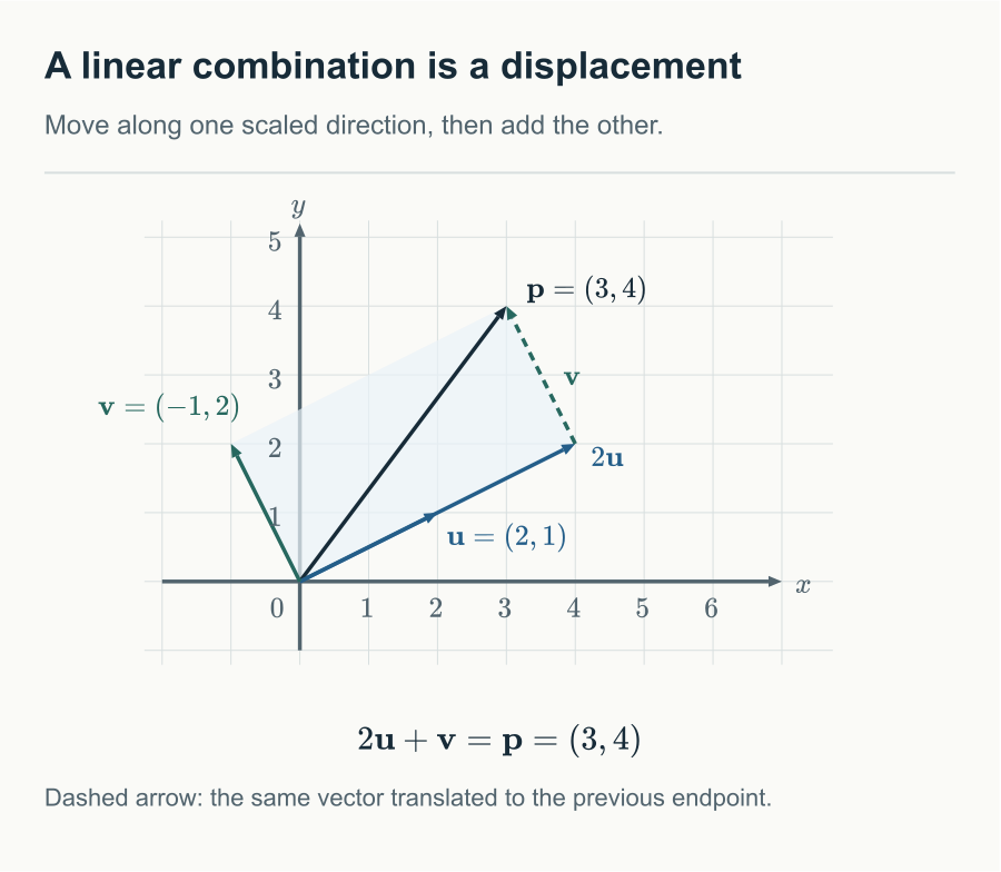
First reach $2\mathbf u=(4,2)$, then make the displacement $\mathbf v=(-1,2)$ to arrive at $\mathbf p=(3,4)$. The dashed arrow is a translated copy of the same displacement, rather than an additional operation.

Coefficients may be negative, zero, or nonintegers, and need not sum to one. For example, $\tfrac12\mathbf u-\mathbf v$ is a linear combination. Adding the restrictions that coefficients are nonnegative and sum to one produces a convex combination, a different question explored in an exercise below.

Which vectors can these directions reach?

One nonzero vector gives a line

As $t$ ranges over the reals, the endpoints of $t\mathbf u$ fill a line through the origin. For $\mathbf u=(2,1)$, this line satisfies $x=2y$.

Positive and negative coefficients extend in opposite directions, while arbitrary real coefficients fill every position between them. Integer coefficients alone would give discrete points, not the whole line. If the given vector is zero, the only reachable point is the origin.

Recovering coefficients from a target

A picture may suggest that arrows can reach a target, but coefficients require an argument. To solve

$$a(2,1)+b(-1,2)=(x,y),$$

compare components. The second equation gives $a=y-2b$. Substitute into the first:

$$2(y-2b)-b=x \quad\Longrightarrow\quad b=\frac{2y-x}{5}.$$

Substitution back gives $a=(2x+y)/5$. Every target has coefficients because these expressions are always defined; they are unique because every solution must equal them.

For the dependent directions $(2,1),(4,2)$, component equations instead give

$$2a+4b=x,\qquad a+2b=y.$$

The first left-hand side doubles the second, requiring $x=2y$. A target violating this condition has no solution. When the condition holds, the equations constrain only $a+2b$, leaving the individual coefficients undetermined. The same directions can therefore produce either no solution or many solutions, depending on the target.

Retain $\mathbf u=(2,1)$, $\mathbf v=(-1,2)$, and dependent direction $\mathbf w=2\mathbf u=(4,2)$. The target $\mathbf p=(3,4)$ violates $x=2y$ and cannot be formed from $\mathbf u,\mathbf w$.

Static comparison: plane and line

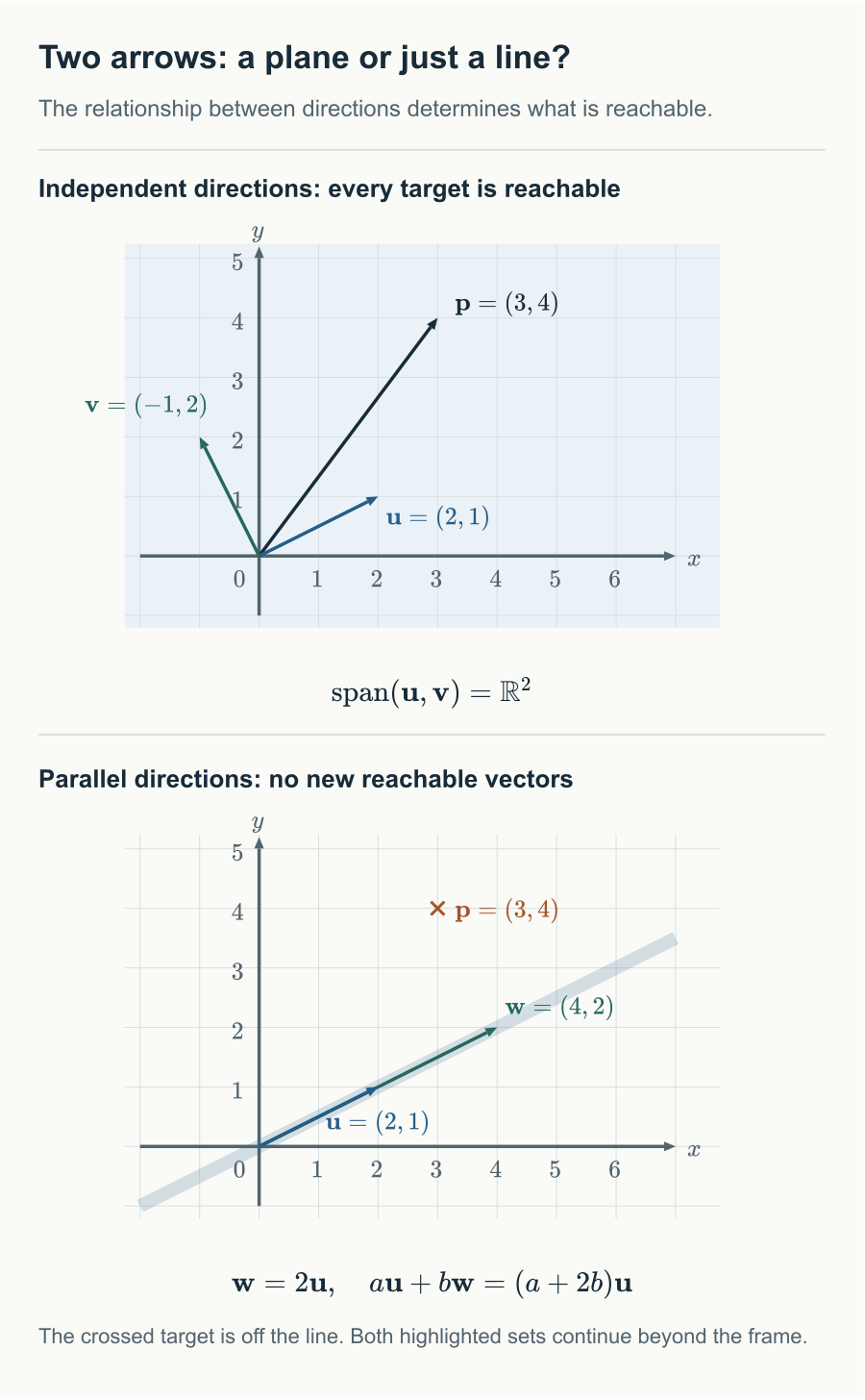
The shading in the upper panel represents the plane; the lower panel highlights only a line. Both continue beyond the frame. The relationship between the directions determines the reachable set, rather than the number of arrows drawn.

Naming the reachable set: span

DefinitionSpan

The set of all real linear combinations of $\mathbf v_1,\ldots,\mathbf v_m$ is their span:

$$\begin{aligned} &\operatorname{span}(\mathbf v_1,\ldots,\mathbf v_m)\\ &\quad=\left\{\sum_{i=1}^m a_i\mathbf v_i:a_i\in\mathbb R\right\}. \end{aligned}$$

We say the vectors span this set, also called the subspace they generate.

The term packages the question we have already answered. Our first pair spans $\mathbb R^2$; our second pair spans a line through the origin.

The scalar field matters. Regarding the complex numbers as a real vector space, $1$ alone spans the real axis and $1,i$ span the complex plane. With complex coefficients allowed, $1$ alone spans $\mathbb C$.

A span in three dimensions

Take $\mathbf r=(1,0,1)$ and $\mathbf s=(0,1,1)$. Then

$$a\mathbf r+b\mathbf s=(a,b,a+b),$$

so every combination lies in the plane $z=x+y$. Conversely, every point in that plane has coefficients $a=x,b=y$. The span is exactly this plane through the origin.

The two directions of the argument matter. Showing that every combination satisfies an equation proves containment; showing that every point satisfying the equation is reachable proves equality.

Adding $\mathbf t=(1,1,2)$ changes nothing because $\mathbf t=\mathbf r+\mathbf s$. Adding $\mathbf e=(0,0,1)$ reaches all of three-dimensional space:

$$(x,y,z)=x\mathbf r+y\mathbf s+(z-x-y)\mathbf e.$$

A new vector enlarges the span precisely when it was not already in the old span.

Redundant directions and unique coefficients

When $\mathbf w=2\mathbf u$, the target $2\mathbf u$ has coefficient pairs $(2,0)$ and $(0,1)$. The relation $2\mathbf u-\mathbf w=\mathbf0$ lets changes in the coefficients cancel.

Our two nonparallel directions instead give each target a unique coefficient pair. This absence of redundancy is called linear independence. Span asks whether a target is reachable; independence asks whether a reachable target has unique coefficients. General definitions, proofs, bases, and dimension follow in vector spaces and bases.

Connecting vectors to matrices and equations

Put the given vectors side by side as matrix columns:

$$A=\begin{pmatrix}2&-1\\1&2\end{pmatrix}.$$

Multiplication by a coefficient column takes a linear combination of those columns:

$$A\begin{pmatrix}a\\b\end{pmatrix} =a\mathbf u+b\mathbf v.$$

The equation $A\mathbf c=\mathbf p$ therefore asks whether the columns can produce the target and which coefficients do so. A solution exists precisely when the target is in the columns’ span. Independent columns guarantee that a solution, if it exists, is unique.

Next, matrices and composition develops the operations before elimination extends this calculation to larger systems.

Exercises

Before calculating, decide whether the question concerns reaching a target or representing it uniquely.

ExerciseScale and add

For $\mathbf u=(2,1)$ and $\mathbf v=(-1,2)$, compute $\tfrac12\mathbf u-\mathbf v$. Explain the negative coefficient geometrically.

Solution

The result is $(2,-3/2)$. Halve $\mathbf u$, then add a displacement of the same length as $\mathbf v$ in the opposite direction.

ExerciseFind the coefficients

Express $(1,3)$ and $(0,1)$ as $a\mathbf u+b\mathbf v$.

Solution

The coefficient pairs are $(1,1)$ and $(1/5,2/5)$, respectively. The second example also shows why allowing integer coefficients alone would miss points in the plane.

ExerciseReachable and unreachable targets

For $\mathbf u=(2,1)$ and $\mathbf w=(4,2)$, which of $(6,3)$ and $(3,4)$ can be reached? Give all coefficient pairs for the former.

Solution

The vector $(6,3)=3\mathbf u$ is reachable. Its coefficients satisfy $a+2b=3$, giving $(a,b)=(3-2t,t)$ for every real $t$. The target $(3,4)$ is unreachable because it does not satisfy $x=2y$.

ExerciseRestricting the coefficients

Suppose $a,b\ge0$ and $a+b=1$. What shape do the vectors $a\mathbf u+b\mathbf v$ form? How does this differ from allowing arbitrary real coefficients?

Solution

Put $b=t$. The vectors are $(1-t)\mathbf u+t\mathbf v$ for $0\le t\le1$, forming the closed line segment between the two endpoints. Without those restrictions, the combinations fill the plane.

ExercisePositions and displacements

Translate $P=(1,2),Q=(4,1)$ by an arbitrary vector $\mathbf h$. Prove that their displacement is unchanged although their position vectors generally change.

Solution

The new displacement is $(Q+\mathbf h)-(P+\mathbf h)=Q-P$. Relative to the original origin, both position vectors increase by $\mathbf h$.

ExerciseA three-dimensional target

Which of $(2,-1,1)$ and $(2,-1,0)$ belongs to $\operatorname{span}((1,0,1),(0,1,1))$?

Solution

The first satisfies $z=x+y$ and has coefficients $(2,-1)$. The second violates the condition. Two three-component vectors do not automatically span three-dimensional space.

References

1. [1] G. Strang, “Independence, Basis and Dimension,” 2011. MIT OpenCourseWare, 18.06SC Linear Algebra, Fall 2011. https://ocw.mit.edu/courses/18-06sc-linear-algebra-fall-2011/pages/ax-b-and-the-four-subspaces/independence-basis-and-dimension/ ↩