Root-Finding and Optimization Through the Fundamental Theorem of Algebra

I was reviewing computational mathematics recently and reached the chapter on root-finding. Before any numerical method, you want to know that a root exists at all, so I went through the proof of the fundamental theorem of algebra again. This time something struck me. The theorem asks whether an equation has a solution, but the proof never solves anything. What it does is look for the lowest point of $|p(z)|$ over the complex plane, and then show that the lowest point must sit at height 0.

In other words, it is an optimization argument.

This post follows that observation. Root-finding and optimization can be rewritten into each other, but each rewrite changes the shape of the problem, its landscape. The fundamental theorem of algebra holds, in the end, because the landscape of $|p|$ over the complex plane is unusually kind: it has no pits other than the roots.

You need very little to follow along: arithmetic with complex numbers, derivatives of one-variable functions, and a bit of partial differentiation. Where complex analysis comes in, I give the intuition first and the statement second. There are two interactive figures below that you can drag and click; they are worth playing with as you read.

Setting the stage: the complex plane as a landscape

A complex number $z=x+iy$ is a point $\left(x,\ y\right)$ in the plane. The horizontal axis is the real axis and the vertical one is the imaginary axis. The modulus

$$|z|=\sqrt{x^2+y^2}$$

is the distance from the point to the origin. The fact used most below is what multiplication does geometrically: when you multiply two complex numbers, their moduli multiply and their arguments (angles from the positive real axis) add. So multiplying by a complex number means scaling and then rotating. Multiplying by $i$, for instance, is a quarter turn counterclockwise, which is also the geometric meaning of $i^2=-1$: two quarter turns point you the opposite way.

A complex polynomial of degree $n$ is

$$p(z)=a_nz^n+a_{n-1}z^{n-1}+\cdots+a_1z+a_0,\qquad a_n\ne0.$$

If $p(z_0)=0$, then $z_0$ is a root of $p$.

TheoremFundamental Theorem of Algebra

Every complex polynomial of degree $n\ge1$ has at least one complex root.

Once you have one root $z_1$, you can write $p$ as $\left(z-z_1\right)q(z)$ and repeat on $q$, so "at least one root" gives "exactly $n$ roots, counted with multiplicity". The only thing to prove is "at least one".

Now look at $p$ from another angle. To every point $z$ of the plane, attach the non-negative number $|p(z)|$ and think of it as the height of the ground there. The whole complex plane becomes a landscape:

• the height is never below 0;
• the places at height 0 are exactly the roots.

So "does $p$ have a root?" becomes "does this landscape reach sea level anywhere?" Below is the landscape of the polynomial this post keeps returning to, $p(z)=z^3-2z+2$. Drag it to rotate.

This interactive figure needs JavaScript.

The three blue dots are the three roots, where the ground drops to 0 like three funnels. The orange curve is the cross-section of the landscape along the real axis; it will come back several times.

A few words from optimization

Before going on, here is the optimization vocabulary we need. Let $f$ be a real-valued function on the plane.

DefinitionGlobal and local minima

A point $z_0$ is a global minimizer of $f$ if $f(z_0)\le f(z)$ for every $z$. It is a local minimizer if this holds for all $z$ in some small neighbourhood of $z_0$.

A local minimum is a small pit in a valley: standing at the bottom, everything around you is higher, yet there may be a deeper valley over the next ridge.

Gradient. For a function of two variables $f\left(x,\ y\right)$, the gradient is the vector of partial derivatives

$$\nabla f=\left(\frac{\partial f}{\partial x},\ \frac{\partial f}{\partial y}\right).$$

It points in the direction in which $f$ increases fastest, and its length is the rate of increase in that direction. So $-\nabla f$ is the steepest way downhill. Gradient descent takes a small step in that direction, again and again:

$$z_{k+1}=z_k-\eta\,\nabla f(z_k),$$

where $\eta>0$ is the step size.

Stationary points and saddles. A point where the gradient vanishes is a stationary point; the ground there is flat. A local minimizer of a smooth function is always stationary, because if the gradient were not zero, a small step along $-\nabla f$ would go lower. A stationary point need not be a minimum, though. The standard example is

$$f\left(x,\ y\right)=x^2-y^2.$$

The gradient vanishes at the origin. Along the $x$ direction the origin is the bottom of a pit; along the $y$ direction it is the top of a ridge. Such a point is a saddle, shaped like a saddle or like a mountain pass between two peaks.

Does a minimum always exist? No. On the open interval $\left(0,\ 1\right)$, $f(x)=x$ creeps towards 0 without ever reaching it. On $[0,\ \infty)$, $e^{-x}$ keeps falling and never bottoms out. The first example leaves out its boundary; the second runs off to infinity. Rule out both and the conclusion holds:

TheoremExtreme Value Theorem (Weierstrass)

A continuous function on a closed and bounded set attains a minimum and a maximum.

"Closed" makes sure boundary points are included; "bounded" makes sure nothing escapes to infinity. In the plane, a closed disc $\{z:|z|\le R\}$ is closed and bounded.

The proof is a minimization problem

With these words, the proof takes three steps. The objective is $f(z)=|p(z)|$.

Step 1: far away, the ground is high. When $|z|$ is large, the modulus of the leading term $a_nz^n$ dwarfs the sum of all the others, so $|p(z)|\to\infty$. Optimizers call this property coercive: the further out you go, the higher it gets, so the lowest point cannot hide at infinity.

Step 2: a lowest point exists. Take a disc large enough that every point outside it is higher than $|p(0)|$. The disc is closed and bounded and $|p|$ is continuous, so by the extreme value theorem $|p|$ has a minimizer $z_0$ in the disc. Points outside the disc are higher than $|p(0)|$, hence higher than $|p(z_0)|$, so $z_0$ is a global minimizer over the whole plane.

Step 3: the lowest point is at height 0. This is the heart of the proof, and it rests on the following lemma.

Lemmad'Alembert's lemma

If $p$ is not constant and $p(z_0)\ne0$, then every neighbourhood of $z_0$, however small, contains a point $z$ with $|p(z)|<|p(z_0)|$.

In optimization terms: a point that is not a root cannot be a local minimum.

Why? Expand $p$ around $z_0$ as a polynomial in $w=z-z_0$, and let $k$ be the first positive power whose coefficient is nonzero:

$$p(z_0+w)=p(z_0)+c\,w^k+(\text{higher powers}),\qquad c\ne0.$$

For small $w$ the higher powers are much smaller than $c\,w^k$, so ignore them for now. To make $|p|$ smaller, the term $c\,w^k$ has to pull $p(z_0)$ towards the origin, which means it should point in the direction of $-p(z_0)$.

This is where the geometry of multiplication does the work. Write $w=re^{i\theta}$. Then $w^k$ has argument $k\theta$, and $c\,w^k$ has argument $\arg c+k\theta$. To make that equal to the argument of $-p(z_0)$, solve for $\theta$, which you can always do: divide the required angle by $k$. With the direction fixed, take $r$ small enough and you get

$$|p(z_0+w)|\approx|p(z_0)|-|c|\,r^k<|p(z_0)|.$$

The simplest example is $p(z)=z^2+1$ at $z_0=0$. Here $p(0)=1$, $k=2$ and $c=1$. To make $w^2$ point towards $-1$, take $w=ir$, since $(ir)^2=-r^2$:

$$p(ir)=1-r^2<1.$$

If only real $w$ were allowed, this step would fail: a real square is never negative, and $p(w)=1+w^2\ge1$. The extra dimension of the complex numbers is exactly what supplies the way down. This point will keep coming back.

Put the three steps together: a lowest point exists, and no point other than a root can be lowest, so the lowest point is a root. The careful estimate that keeps the higher powers under control is in my note on complex numbers; I will not repeat it here.

This line of argument has a winding history. d'Alembert gave the lemma in 1746 but took the existence of a minimum for granted. Gauss's 1799 doctoral thesis criticized the earlier proofs, d'Alembert's among them. Argand, in work from 1806 and 1814, organized the argument around the minimum of $|p|$ in the form we use today, and Cauchy followed it in his 1821 Cours d'analyse. The extreme value theorem behind Step 2, however, only became fully rigorous with Weierstrass in the second half of the nineteenth century [1][1] H. D. Ebbinghaus, H. Hermes, F. Hirzebruch, M. Koecher, K. Mainzer, J. Neukirch, A. Prestel, and R. Remmert, Numbers. Springer, 1991. Chapter 4, R. Remmert, The Fundamental Theorem of Algebra., [2][2] B. Fine and G. Rosenberger, The Fundamental Theorem of Algebra. Springer, 1997.. So the most analytic part of this proof is precisely the most basic existence theorem of optimization.

Two ways to translate

Seen this way, root-finding and optimization were already joined by two bridges.

From root-finding to optimization. To solve a system $F(x)=0$, minimize

$$\phi(x)=\tfrac{1}{2}\|F(x)\|^2.$$

Here $\|F\|$ is the length of the vector. Since $\phi\ge0$, and $\phi(x)=0$ exactly when $F(x)=0$, any minimizer with minimum value 0 is a root. The factor $\tfrac{1}{2}$ just tidies up the derivative. Nonlinear least squares and the Gauss–Newton method both start here.

From optimization to root-finding. To minimize a smooth function $f$, recall that every local minimizer satisfies

$$\nabla f(x)=0.$$

That is a system of equations. Fermat used a similar idea to find extrema in the 1630s. Newton's method for optimization is simply Newton's method for finding a root of $\nabla f$.

Both bridges work, but the view from the other side is different. A concrete polynomial shows how.

An example: a false pit on the real line

Take again

$$p(x)=x^3-2x+2.$$

It is an old friend from numerical analysis courses: Newton's method started at 0 jumps between 0 and 1 forever. It has one real root, about $-1.7693$, and a pair of complex conjugate roots $0.8846\pm0.5897i$.

First stay on the real line and find the root by minimizing $p(x)^2$. The derivative $p'(x)=3x^2-2$ vanishes at $x=\pm\sqrt{2/3}\approx\pm0.8165$. Call $x_0=\sqrt{2/3}$. At this point $p$ has a local minimum of about 0.911, which is not 0.

That is a false pit: a local minimizer of $p^2$ that is not a root. Run gradient descent on the real line from any start to the right of $-0.8165$, and you slide into this pit and stay there. Rewriting the problem as optimization over the reals alone has lost what root-finding was asking for.

$x^2+1$ makes the same point more bluntly: its lowest point on the real line is $x=0$, at height 1, and it has no real root at all.

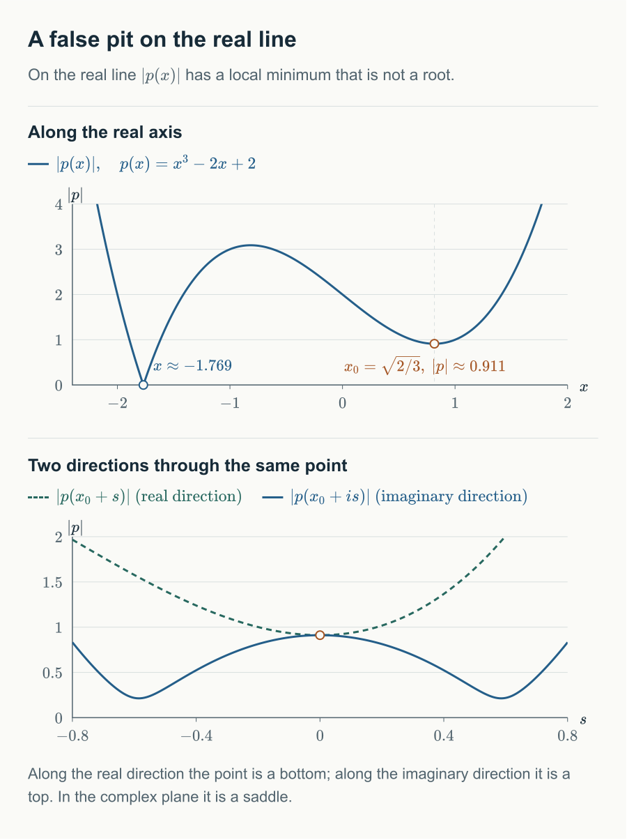
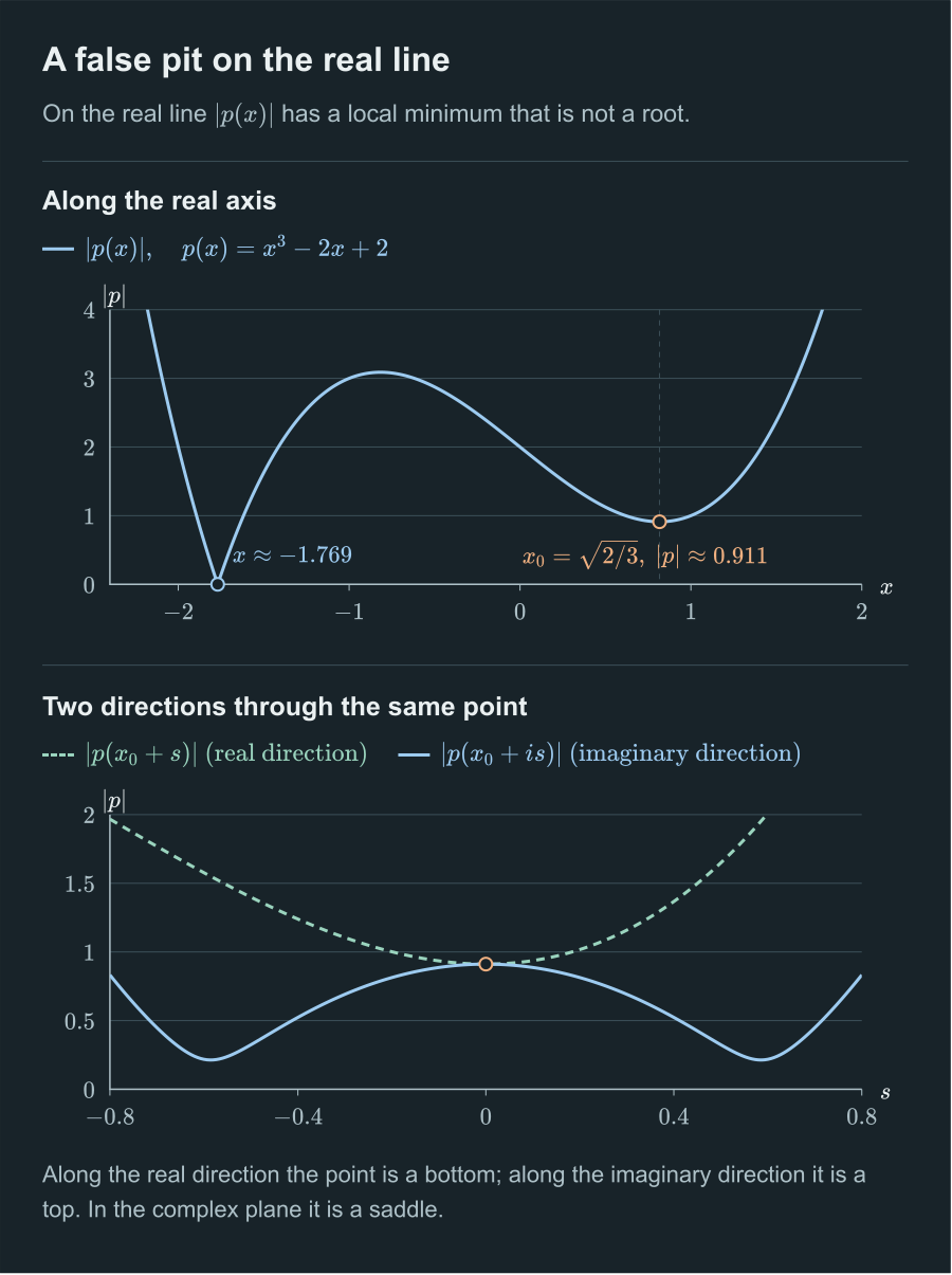
The top panel is $|p(x)|$ on the real line: the true root on the left, the false pit on the right. The bottom panel goes through the same point $x_0$ and compares what $|p|$ does along the real and the imaginary directions. The next section explains it.

In the complex plane, the false pit is a saddle

Now put $x_0$ into the complex plane. Since $p'(x_0)=0$, the linear term of the expansion vanishes and the first nonzero term is quadratic:

$$p(x_0+w)\approx 0.911+2.449\,w^2.$$

This is d'Alembert's lemma with $k=2$. Moving along the real axis, $w$ is real, $w^2>0$, and $|p|$ grows, so on the real line $x_0$ looks like the bottom of a pit. But to make $2.449\,w^2$ point along the negative real axis, all you need is a purely imaginary $w$. With $w=is$,

$$p(x_0+is)\approx 0.911-2.449\,s^2,$$

and $|p|$ goes down.

What looks like the bottom of a pit from the real line is, in the complex plane, only a mountain pass: uphill along the real axis, downhill along the imaginary axis, just like the saddle of $x^2-y^2$ above. Go back to the 3D landscape and press "Real-axis profile". The surface is cut along the real axis and the front edge is the real-axis curve, pit at $x_0$ included. Rotate slowly and you will see the surface behind the pit falling away.

$x^2+1$ behaves the same way. At $z=0$, to make $w^2$ point towards $-1$, take $w=\pm i$. Walking downhill along the imaginary axis leads straight to its two roots $\pm i$.

This gave me a more concrete feel for why the fundamental theorem of algebra has to live in the complex numbers. The counterexamples over the reals are not missing a few roots by accident; their landscapes have pits. What the complex numbers do is turn every such pit into a saddle.

Why the complex plane has no false pits

The previous section looked at a single point. To see that the same holds everywhere, we need a more global tool: harmonic functions.

DefinitionHarmonic function

A real function $u\left(x,\ y\right)$ of two variables is harmonic if

$$\frac{\partial^2u}{\partial x^2}+\frac{\partial^2u}{\partial y^2}=0.$$

The intuition behind this condition is simple: the bending in the $x$ direction is exactly opposite to the bending in the $y$ direction. If the function curves upward along $x$ (positive second derivative), it must curve downward along $y$. A strict local minimum needs upward curvature in every direction, which contradicts the condition.

An equivalent way to say this is the mean value property: a harmonic function's value at a point equals its average over any small circle centred there. If a point were lower than everything around it, the average could not equal its value. So a harmonic function, unless constant, has no local minima and no local maxima.

The fact that matters here is that wherever $p(z)\ne0$, the function $\log|p(z)|$ is harmonic. Locally it is the real part of the analytic function $\log p(z)$, and the real part of any analytic function satisfies the equation above (this follows directly from the Cauchy–Riemann equations). Since $\log$ is increasing, it does not change where the ground is high or low. Therefore:

• $|p|$ has no local minima away from its zeros. This is the minimum modulus principle of complex analysis;
• every stationary point of $|p|$ that is not a root, that is, every point with $p'(z)=0$ but $p(z)\ne0$, must be a saddle.

Check it at $x_0$: along the real axis the second derivative of $\log|p|$ is $p''(x_0)/p(x_0)\approx5.38>0$, curving upward. The harmonic condition then says the second derivative along the imaginary axis is $-5.38$, curving downward. This matches the expansion in the previous section.

From this angle, d'Alembert's lemma is the local face of a more general fact. A non-constant analytic function maps every small neighbourhood onto an open set around $p(z_0)$ (the open mapping theorem), and that open set naturally contains points closer to the origin.

Here is how this looks for an algorithm. Written as a complex number, the gradient of $|p|^2$ is

$$2\,\overline{p'(z)}\,p(z),$$

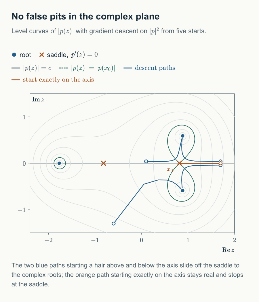
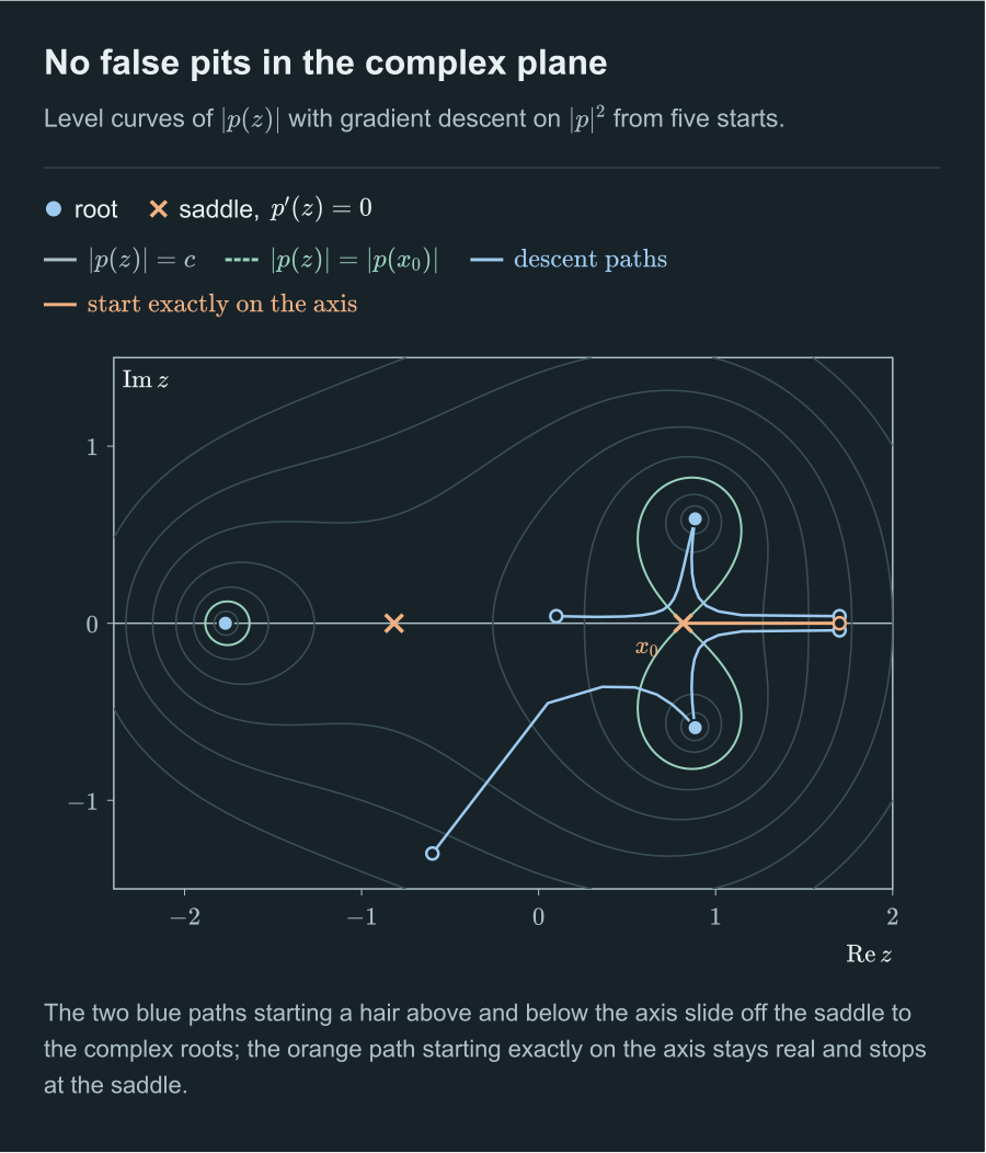
which vanishes only at the roots and at the zeros of $p'$. I scattered 2000 random starting points over $[-2,\ 2]\times[-2,\ 2]$ and ran gradient descent on $|p(z)|^2$ with step size $\eta=0.002$. Every one of the 2000 starts converged to one of the three roots, with a largest residual $|p|$ on the order of $10^{-14}$. The pit that traps most starts on the real line leaves no trace in the complex plane.

You can try this yourself below: click anywhere in the plane to start, and watch gradient descent find its way. The thin lines are level curves of $|p|$, the background turns a deeper blue as you approach a root, and the dashed figure eight is the level curve through the saddle $x_0$.

This interactive figure needs JavaScript.

Two presets are worth comparing: "1.7" and "1.7+0.04i". There is exactly one way to fail: start exactly on the real axis. The coefficients of $p$ are real, so the gradient on the real axis is real too, the iterates never leave the axis, and they stop at the saddle $x_0$. Move the start up or down by a hair and the path slides past the saddle into a complex root. A random start almost never lands exactly on the real axis, which is why all 2000 starts succeeded.

Static figure: five gradient descent paths

The same idea inside numerical methods

Numerical methods use this connection all the time, usually without saying so. First a quick reminder of Newton's method.

Newton's method. At the current point $z_k$, approximate $p$ by its tangent line: $p(z)\approx p(z_k)+p'(z_k)(z-z_k)$. Setting the right-hand side to zero gives the next point

$$z_{k+1}=z_k-\frac{p(z_k)}{p'(z_k)}.$$

For a system $F(x)=0$, the derivative becomes the Jacobian matrix $J$, the matrix of all partial derivatives $\partial F_i/\partial x_j$, and the Newton step becomes $x_{k+1}=x_k-J^{-1}F(x_k)$. Near a root Newton's method converges very fast; far from one it can jump around wildly.

Back to $p(z)=z^3-2z+2$. Plain Newton started at 0 gives

$$0\ \to\ 1\ \to\ 0\ \to\ 1\ \to\ \cdots$$

Watch $|p|$: $|p(0)|=2$, $|p(1)|=1$, then back to 2. The jump from 1 back to 0 doubles $|p|$.

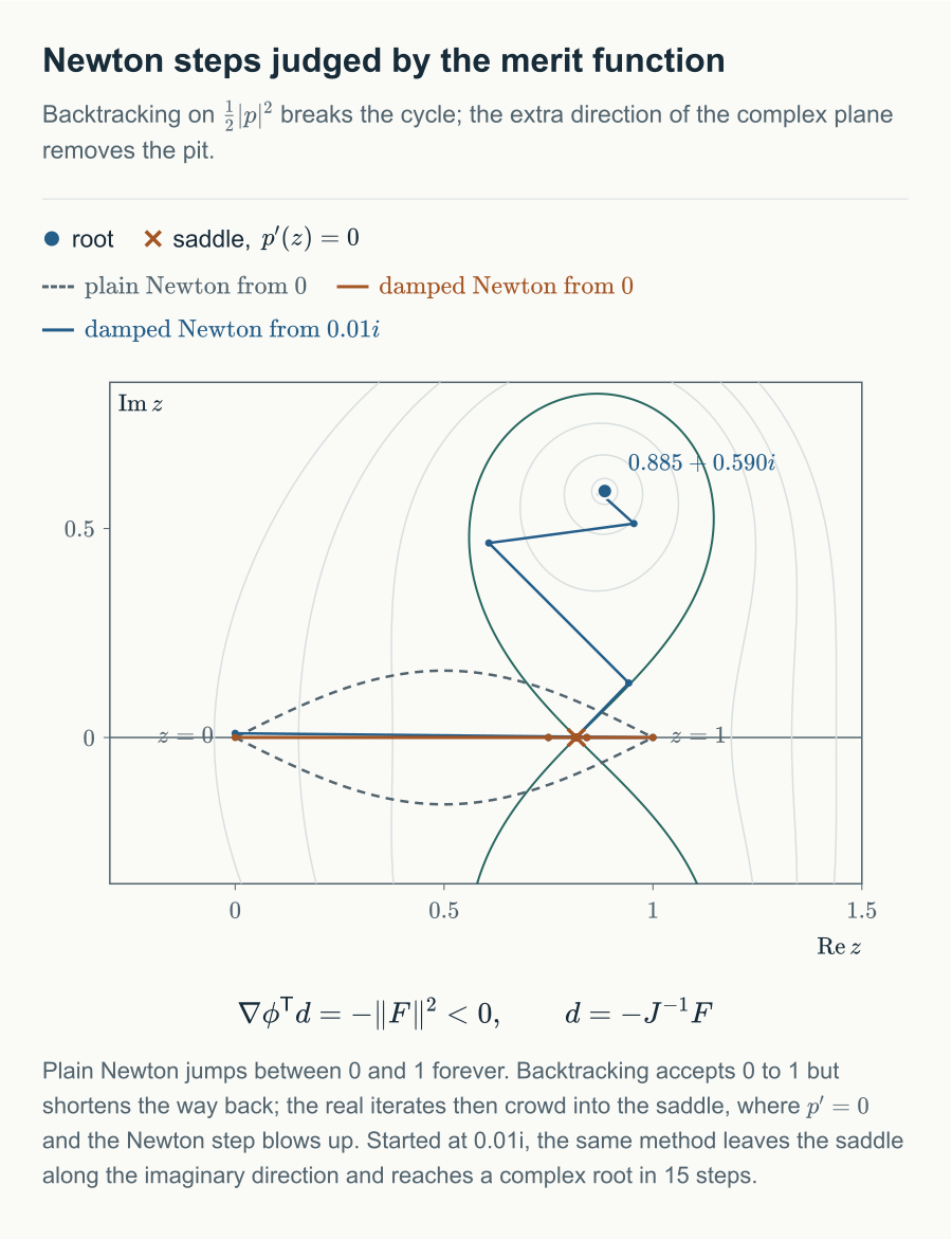
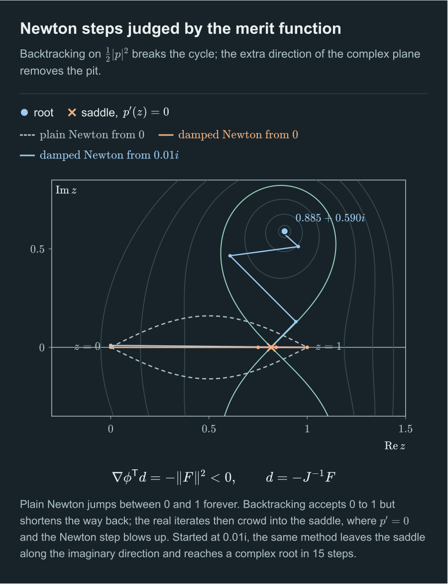
Merit functions and backtracking. A natural fix is to give Newton's method a yardstick for whether a step made things better. The yardstick is the $\phi=\tfrac{1}{2}|p|^2$ from before, which optimizers call a merit function. Try the full Newton step first; if $\phi$ has not dropped enough, halve the step and try again, until it has. This is backtracking line search, and Newton's method with it is damped Newton.

It does break the cycle. The jump from 0 to 1 lowers $|p|$ from 2 to 1 and is accepted. Jumping from 1 back to 0 would double $|p|$, so backtracking cuts the step to a quarter and lands at 0.75.

When I actually ran it, though, a new problem appeared. The iterates crept towards 0.8165, the false pit $x_0$ from before. There $p'=0$, so the Newton step $p/p'$ becomes infinitely long, and backtracking has to shrink it more and more until the method barely moves. It sat beside the pit for about ten steps; eventually rounding error let one step slip out by chance, and it landed on the real root $-1.7693$. The method deserves no credit for that. As long as everything is computed in real arithmetic, the iterates cannot leave the real axis, and on the real axis the pit is real.

Start at $0.01i$ instead and the story changes. The iterates again approach $x_0$, then slide down the pass in the imaginary direction and converge to the complex root $0.8846+0.5897i$ in 15 steps. The merit function broke the cycle, and the extra direction of the complex plane removed the pit.

In the figure above, switch the method to "Damped Newton" or "Plain Newton" and use the presets "0" and "0.01i" to see both outcomes. The "step fraction" in the status line is the part of the Newton step that backtracking actually kept.

Static figure: three Newton paths

Why is it sensible to judge Newton's method by a merit function? There is a clean fact behind it. The Newton direction is $d=-J^{-1}F$, and the gradient of the merit function is $\nabla\phi=J^{\mathsf T}F$. The directional derivative along the Newton direction is their inner product:

$$\nabla\phi^{\mathsf T}d=-F^{\mathsf T}JJ^{-1}F=-\|F\|^2<0.$$

As long as we are not at a root and $J$ is invertible, the Newton direction always points downhill for $\phi$; a full step may just be too long, and backtracking shortens it. Conversely, the places where such methods really go wrong are exactly the points where $J$ is singular: there the Newton direction stops making sense, and the iteration can stall at a point that is not a root [3][3] J. Nocedal and S. J. Wright, Numerical Optimization, 2nd ed. Springer, 2006.. The $x_0$ above is such a point.

Root-finding algorithms borrow optimization's yardstick to judge progress, in the same spirit as d'Alembert's lemma: if you are not at a root, there should be a way down. Systems of equations in higher dimensions are not as lucky as the complex plane, though. $\|F\|^2$ can have genuine false pits, local minimizers with $J^{\mathsf T}F=0$ but $F\ne0$. When Gauss–Newton or Levenberg–Marquardt get stuck, this is often why. The real-line $x^3-2x+2$ is the smallest model of that failure.

The converse fails: not every root-finding problem is optimization

The two bridges are not symmetric.

Going from optimization to root-finding always produces a system of the form $\nabla f=0$. But for a vector field $F$ to be a gradient $\nabla f$, it must satisfy a condition. In the plane, if $F=\left(F_1,\ F_2\right)=\nabla f$, then

$$\frac{\partial F_1}{\partial y}=\frac{\partial^2f}{\partial y\,\partial x}=\frac{\partial^2f}{\partial x\,\partial y}=\frac{\partial F_2}{\partial x},$$

because mixed partial derivatives of a smooth function do not depend on the order of differentiation. In matrix language, the Jacobian of $F$ must be symmetric. On a region without holes (a simply connected region) the condition is also sufficient. Most systems of equations fail it, so root-finding is much broader than finding stationary points.

The simplest counterexample comes from games. Picture two players: one controls $x$ and wants $xy$ as small as possible; the other controls $y$ and wants it as large as possible. That is

$$\min_x\max_y\ xy.$$

The equilibrium is the origin: neither player gains by moving alone. It is also a root of the system $F\left(x,\ y\right)=\left(y,\ -x\right)=0$, where the first component $y$ is the partial derivative of $xy$ in $x$, and the second is the partial derivative in $y$ with its sign flipped, because the $y$ player is climbing. The Jacobian of this $F$ is antisymmetric, so $F$ is not the gradient of any function.

The most direct algorithm lets both players move at once, $x$ down its gradient and $y$ up its own. This is gradient descent-ascent:

$$x_{k+1}=x_k-\eta\,y_k,\qquad y_{k+1}=y_k+\eta\,x_k.$$

Each step rotates the point $\left(x_k,\ y_k\right)$ by a small angle and stretches it by $\sqrt{1+\eta^2}$. With $\eta=0.1$ and starting from $\left(1,\ 0\right)$, after 100 steps the distance to the origin is about 1.64, spiralling outward. There is no landscape here, so there is no downhill. Training a generative adversarial network (GAN) is at heart a min-max problem of this kind, and some of its circling and oscillation comes from exactly this.

So the more accurate statement is this: optimization is a special case of root-finding (root-finding for gradient fields), while root-finding can always be recast as optimization through $\|F\|^2$, at the price of pits the original problem never had.

Back to learning

Part of why this matters to me is how closely it resembles current theory in machine learning.

The easiest objectives in optimization are convex functions: bowl-shaped, so every local minimum is global and there are no false pits. Almost every objective in deep learning is non-convex, so in principle gradient descent could get stuck in a bad local minimum at any time. In practice it usually works well. Over the past decade a line of research has looked for problems that are non-convex but have a benign landscape: every local minimum is global, and every other stationary point is a saddle with a way down. Matrix completion [4][4] R. Ge, J. D. Lee, and T. Ma, “Matrix Completion has No Spurious Local Minimum,” arXiv:1605.07272, 2016. https://arxiv.org/abs/1605.07272, dictionary learning and phase retrieval [5][5] J. Sun, Q. Qu, and J. Wright, “When Are Nonconvex Problems Not Scary?,” arXiv:1510.06096, 2015. https://arxiv.org/abs/1510.06096 have all been shown to belong to this class. Add results showing that gradient descent almost never stops at a strict saddle [6][6] J. D. Lee, M. Simchowitz, M. I. Jordan, and B. Recht, “Gradient Descent Converges to Minimizers,” arXiv:1602.04915, 2016. https://arxiv.org/abs/1602.04915, and you can explain why simple algorithms are enough. In the experiment above, only paths that start exactly on the real axis stop at the saddle, a small instance of that result: the real axis is a line in the complex plane, and a random start lands on it with probability 0.

Lay out the structure of these arguments and it is exactly Argand's: the objective grows to infinity far away, so a minimum exists; every stationary point that is not globally optimal has a descent direction, so local optima are global.

In one detail the fundamental theorem of algebra is actually stronger. Machine learning results usually require saddles to be strict: the Hessian (the matrix of second partial derivatives) has at least one negative eigenvalue, so at least one direction curves downward and second-order information finds the way down. In d'Alembert's lemma, however, $k$ can be 3, 4 or more. Take $p(z)=z^3+1$ at $z=0$: here $k=3$, every second derivative vanishes, and the point is a "monkey saddle" (three ways down, one of them for the monkey's tail). Second-order information sees no descent direction at all. The lemma finds the way using the $k$-th order term and a $k$-th root. For general functions, degenerate saddles of this kind are much harder to handle; the structure of polynomials makes them easy.

Closing

Looking back, the name of the theorem is a little misleading. Its proof uses almost no algebra. It uses two facts from analysis: a continuous function on a closed and bounded set attains its minimum, and complex numbers have $k$-th roots. The first guarantees that a lowest point exists; the second guarantees that away from it there is always a way downhill.

When I first learned it, I treated it as nothing more than the premise "a root exists" and moved on. Reading it again, it already previews much of what comes later: root-finding can become a search for the lowest point; whether that search succeeds depends on whether the landscape has false pits; and the right space, with the right structure, can make the false pits disappear.

References

1. [1] H. D. Ebbinghaus, H. Hermes, F. Hirzebruch, M. Koecher, K. Mainzer, J. Neukirch, A. Prestel, and R. Remmert, Numbers. Springer, 1991. Chapter 4, R. Remmert, The Fundamental Theorem of Algebra. ↩
2. [2] B. Fine and G. Rosenberger, The Fundamental Theorem of Algebra. Springer, 1997. ↩
3. [3] J. Nocedal and S. J. Wright, Numerical Optimization, 2nd ed. Springer, 2006. ↩
4. [4] R. Ge, J. D. Lee, and T. Ma, “Matrix Completion has No Spurious Local Minimum,” arXiv:1605.07272, 2016. https://arxiv.org/abs/1605.07272 ↩
5. [5] J. Sun, Q. Qu, and J. Wright, “When Are Nonconvex Problems Not Scary?,” arXiv:1510.06096, 2015. https://arxiv.org/abs/1510.06096 ↩
6. [6] J. D. Lee, M. Simchowitz, M. I. Jordan, and B. Recht, “Gradient Descent Converges to Minimizers,” arXiv:1602.04915, 2016. https://arxiv.org/abs/1602.04915 ↩