Relations and Order

NBG Set Theory and Binary Relation

In this chapter, we will discuss further topics on set theory, or more specifically, relations. With set as tool, we can categorize things and try to build connections between them, like defining a function from a preimage to an image. Relation is a superset , i.e., generalization of function, which is crucial to topics that we will discuss later in this chapter.

In real life, relation is referred to as some connections between one person or one group of people to the other.

1. Imagine a list of students and their grades in a class. Each student (let's say, by their student ID) is linked to a specific grade. This "student-to-grade" pairing is an example of a functional relation, because every student has one and only one grade assigned.

2. Consider the relationship "has the same birthday as" among people. If person A has the same birthday as person B, and person B has the same birthday as person C, then person A also has the same birthday as person C. This relationship is an equivalence relation because it's reflexive (everyone has the same birthday as themselves), symmetric (if A shares a birthday with B, then B shares a birthday with A), and transitive (if A shares a birthday with B, and B with C, then A shares a birthday with C).

3. Numerical heights have the usual order $\le$. On books themselves, “has height at most” is only a preorder: two different books can have the same height, so antisymmetry may fail.

The notion is still quite similar in the context of mathematics. From many examples we can see this. Like all the mathematical operations we have defined, the mapping in a function, congruence... To sum up, relation is am abstract topic, yet not hard to understand, since it can be related to the material world easily.

From elementary sets to classes

Naive Set Theory introduced ordinary set constructions informally, with specified source sets. It did not assume that every description defines a set. The contradictory principle is unrestricted comprehension: treating the Russell collection $R=\{x:x\notin x\}$ as a set gives $R\in R$ if and only if $R\notin R$.

Here we introduce the language of NBG (von Neumann–Bernays–Gödel) set theory to discuss both sets and larger collections. This is background for the chapter, not a requirement for defining an order on an ordinary set: a relation on a set $A$ is already represented by a subset of $A\times A$ [1][1] T. Banakh, “Classical Set Theory: Theory of Sets and Classes,” arXiv:2006.01613, 2026. Version 6, August 15, 2026; NBG sets, classes, and class existence. https://arxiv.org/abs/2006.01613.

DefinitionSets and proper classes

In a one-sorted presentation of NBG, the objects are classes, and every member of a class is a set. A class that is a member of another class is a set; a class that is not a set is a proper class. Thus every set is a class, but proper classes cannot themselves be elements.

The class $V$ of all sets and the class of all ordinals are proper classes. Allowing them as classes does not turn them into sets or permit arbitrary classes as members.

Extensionality and elementary class comprehension

AxiomExtensionality of classes

Classes with the same members are equal:

$$\forall A\,\forall B\bigl(\forall x\,(x\in A\leftrightarrow x\in B)\to A=B\bigr).$$

AxiomElementary class comprehension

Let $P(x)$ be a formula whose quantified variables range only over sets; fixed set and class parameters may occur. There is a class

$$C=\{x:x\text{ is a set and }P(x)\}.$$

Thus $u\in C$ exactly when $u$ is a set and $P(u)$ holds. This is a schema restricted to formulas with set quantifiers, not a rule for arbitrary formulas quantifying over classes.

These principles explain the class constructions used below; they are not the complete NBG axiom list. In particular, introducing class notation alone does not settle every set-existence question. Choice conventions also vary between presentations and must be stated when they are needed.

Properties and Operations of Class

Since the definition of Class and set are related, there are a lot of overlap in their properties. The union and intersection of two classes are defined in exactly the same way as the union and intersection of two sets in naïve set theory: if $A$ and $B$ are classes, then

$$$$ $$\begin{aligned} A \cup B &= \{x : (x \in A) \vee (x \in B)\}, \\ A \cap B &= \{x : (x \in A) \wedge (x \in B)\}. \end{aligned}$$ $$$$

So a set $x$ is a member of $A \cup B$ if and only if it is a member of either $A$ or $B$ (or both); $x$ is a member of $A \cap B$ if and only if it is a member of both $A$ and $B$.

The usual properties of these unions and intersections are established as in naïve set theory. Namely, we have the properties known as idempotence,

$$$$ $$\begin{aligned} \forall X(X \cup X = X), \quad \forall X(X \cap X = X), \end{aligned}$$ $$$$

associativity,

$$$$ $$\begin{aligned} \forall X \forall Y \forall Z (X \cup (Y \cup Z) = (X \cup Y) \cup Z), \\ \forall X \forall Y \forall Z (X \cap (Y \cap Z) = (X \cap Y) \cap Z), \end{aligned}$$ $$$$

commutativity,

$$$$ $$\begin{aligned} \forall X \forall Y (X \cup Y = Y \cup X), \quad \forall X \forall Y (X \cap Y = Y \cap X), \end{aligned}$$ $$$$

and distributivity,

$$$$ $$\begin{aligned} \forall X \forall Y \forall Z (X \cup (Y \cap Z) = (X \cup Y) \cap (X \cup Z)), \\ \forall X \forall Y \forall Z (X \cap (Y \cup Z) = (X \cap Y) \cup (X \cap Z)). \end{aligned}$$ $$$$

DefinitionClass Complement

We write $x \notin y$ as an abbreviation for $\neg(x \in y)$. Then for each class $A$ we define the complement of $A$ to be the class

$$$$$$\begin{aligned} \sim A = \{x : x \notin A\}. \end{aligned}$$$$$$

DefinitionClass Difference

For two classes $A$ and $B$, the difference $A~B$ is defined as:

$$A\sim B \text{ or } A-B=\{x:(x\in A)\land(x\not\in B)\}=A\cap(\thicksim B).$$

Also, note that double negation and De Morgan's Law also work for class.

As what we have discussed in set theory that there exist some empty sets, we also have null class and universe class.

DefinitionEmpty and Universal Classes

Empty class $\emptyset$ and universe class $V$ are defined by

$$\emptyset=\{x:x\neq x\}\ \ \ V=\{x:x=x\}.$$

Classes also have their exclusive operations, including intersection and union.

DefinitionUnion and Intersection of Classes

Let $A$ be a class; the union and intersection of the class $A$ are the classes

$$\begin{array}{rcl}\bigcup A&=&\{x:(\exists y)((y\in A)\land(x\in y))\},\\ \bigcap A&=&\{x:(\forall y)((y\in A)\to (x\in y))\}\end{array}$$

Where $x$ is a set and $y$ is a class.

Thus a class $C$ belongs to $\bigcup A$ if and only if $C$ is a set and $C$ belongs to at least one of the members of $A;C$ belongs to $\bigcap A$ if and only if $C$ is a set and $C$ belongs to every member of $A.$

The definition is quite different from intersection and union of sets, as class is a generalization of set from higher level abstraction. Also, the intersection and union for sets are binary operations, while unary for one class.

Below is a brief comparison.

Set Union and Intersection:

1. For two sets $A$ and $B$, their union $A \cup B$ is the set of all elements that belong to either $A$ or $B$. Formally: $A \cup B = \{x : x \in A \lor x \in B\}$.

2. For two sets $A$ and $B$, their intersection $A \cap B$ is the set of all elements that belong to both $A$ and $B$. Formally: $A \cap B = \{x : x \in A \land x \in B\}$.

Class Union and Intersection:

1. For a class $A$, the class union $\bigcup A$ is the set of all elements $x$ such that there exists a class $y$, where $y$ is a member of $A$, and $x$ is an element of $y$. Formally: $\bigcup A = \{x : (\exists y)((y \in A) \land (x \in y))\}$.

2. For a class $A$, the class intersection $\bigcap A$ is the set of all elements $x$ such that for every class $y$, if $y$ is a member of $A$, then $x$ is an element of $y$. Formally: $\bigcap A = \{x : (\forall y)((y \in A) \to (x \in y))\}$.

Comparison:

1. Set union and intersection operate on two sets, while class union and intersection operate on all member sets of a class.

2. Set union includes elements that are in either $A$ or $B$, while class union includes elements that are in at least one member of $A$.

3. Set intersection includes elements that are in both $A$ and $B$, while class intersection includes elements that are in all members of $A$.

4. The result of set union and intersection is always a set, while the result of class union and intersection is not necessarily a set , but more likely a class that contains sets.

By comparing these concepts, we can see that class union and intersection are generalizations of set operations at a higher level of abstraction. They allow us to perform operations on the member sets of a class to obtain new sets, which is particularly useful when studying advanced topics in mathematical foundations and set theory.

There are several lemmas related to intersection and union of class.

LemmaEmpty-Class Union and Intersection

$\bigcap \emptyset= V$ and $\bigcup \emptyset= \emptyset.$

Proof

Let $C$ be a class. Then we have

$$C \in \bigcap \emptyset \iff C \text{ is a set and } C \text{ belongs to every member of } \emptyset$$

Since $\emptyset$ does not literally have any member.

$$\iff C \text{ is a set}$$

Any set is a member of universe class

$$\iff C \in V.$$

Thus

$$\bigcap \emptyset = V$$

by the Axiom of Extensionality.

Again let $C$ be a class. Then

$$C \in \bigcup \emptyset \iff C \text{ is a set and there is a member } x \text{ of } \emptyset \text{ such that } C \in x$$$$\iff C \in \emptyset$$

(since $\emptyset$ has no members).

So

$$\bigcup \emptyset = \emptyset$$

by the Axiom of Extensionality.

The inclusive relation of class is very similar to set.

DefinitionClass Inclusion

If $A$ and $B$ are classes such that every member of $A$ is also a member of $B$, i.e., such that we have

$$\forall x ((x \in A) \to (x \in B)),$$

we say that $A$ is included in $B$, $B$ includes $A$ or $A$ is a subclass of $B$, and we write $A \subseteq B$ or $B \supseteq A$. (If $A$ is a set and $A \subseteq B$ we say that $A$ is a subset of $B$.) If $A \subseteq B$ and there is at least one set $b$ such that $b \in B$ but $b \not\in A$, we say that $A$ is properly included in $B$, $B$ properly includes $A$ or $A$ is a proper subclass of $B$, and we write $A \subset B$ or $B \supset A$.

We can also extend power set to power class. For every class $A$ we define the power class $P(A)$ of $A$ to be the class of all subsets of $A$, i.e., $P(A) = \{x : x \subseteq A\}$. This brings us to another axiom in NBG set theory.

AxiomPower Set Axiom

For every set $x$ there exists a set $y$ such that $u \in y$ if and only if $u \subseteq x$.

The Power Set Axiom thus asserts that every subclass $u$ of a set $x$ is actually a set (since it is an element of the set $y$ whose existence is asserted by the axiom) and furthermore that the power class $P(x)$ of a set $x$ is also a set (and so is usually referred to as the power set of $x$).

The rest of the axioms are as follows.

AxiomPairing Axiom

For all sets $x$ and $y$ the class $\{z : (z = x) \vee (z = y)\}$ is a set.

The set $\{z : (z = x) \vee (z = y)\}$ is denoted by $\{x, y\}$ and such a set is called an unordered pair. If $x = y$ the unordered pair $\{x, y\}$ is denoted by $\{x\}$ and is called singleton $x$.

RemarkUnordered Pairs

In set theory, an unordered pair refers to a collection of two elements in which the sequence of the elements does not matter. This is represented as $\{a, b\}$, indicating a set that contains exactly two distinct elements $a$ and $b$. The fundamental property of unordered pairs is that $\{a, b\} = \{b, a\}$, asserting that the order of elements is immaterial.

The concept of an unordered pair is not limited to sets; it extends to classes in certain set theories that distinguish between sets and proper classes. While sets are collections of elements that themselves can be elements of other sets, proper classes are collections too large to be sets and hence cannot be elements of other collections. Nonetheless, the notion of grouping two objects into an unordered pair applies analogously, symbolizing the collection of those objects without regard to order.

AxiomUnion Axiom

For every set $x$ the class $\bigcup x$ is a set.

We can also extend Cartesian Product to class. Let $a$ and $b$ be sets. Then the set $\{\{a\},\{a,b\}\}$ is denoted by $(a,b)$ and is called the ordered pair with first coordinate $a$ and second coordinate $b$. Lét $A$ and $B$ be classes; then the Cartesian product of $A$ and $B$ is the $c$lass

$$A\times B=\{t:(\exists x)(\exists y)((x\in A)\land(y\in B)\land(t=(x,y)))\},$$

i.e. $A\times B$ is the class of all ordered pairs with first coordinate in $A$ and second coordinate in $B.$

If $P(x,y)$ is an open sentence involving the free variables $x$ and $y$ we shall allow ourselves to write

$$\{(x,y):P(x,y)\}$$

as an abbreviation for

$$\{t:(\exists x)(\exists y)((t=(x,y))\land P(x,y))\}.$$

So we can abbreviate the definition of $A\times B$ to

$$A\times B=\{(x,y):(x\in A)\wedge(y\in B)\}.$$

Binary Relations, Composition and Inverse

In mathematics, the most fundamental and ubiquitous type of relation is the binary relation. This term refers to a relationship between two objects or sets. We understand that a 'set' may encompass any concept, not solely in the mathematical sense but also in a material one. Relations may exist objectively between certain objects and not at all for others. Similarly, objects or sets of objects, which exist objectively, hold the potential for an infinite number of relationships with one another. This perspective can seem philosophically abstract, positing that any scenario is conceivable. However, we can convey this more clearly. Recall our discussion of the Cartesian product as a set extension, where we consider two sets, $A$ and $B$. These sets could represent any discernible entity or indiscernible concept. Theoretically, there could be countless relationships among all elements of these sets, and the capacity of two sets to form a Cartesian product is indicative of a general type of relationship. Consequently, the elements of the power set $P(A \times B)$ exemplify all possible cases of a certain kind of relationship.

A vivid mathematical example is the definition of Euclidean spaces, where an infinite number of subspaces can be defined, each representing a unique binary relation within the space.

We first introduce the definition of a binary relation in terms of sets.

DefinitionBinary Relations

A Binary Relation $R$ from a set $A$ to a set $B$ is a subset of the Cartesian product $A \times B$. For elements $a \in A$ and $b \in B$, if the pair $(a, b)$ belongs to the subset $R$, then we say $a$ is related to $b$ by the relation $R$, denoted as $aRb$, whose negation is $a\not R b$.

In last section, we introduced the higher abstraction of sets, which is class. Classes also have Cartesian product,thus, we can give a general definition to all relations using class.

DefinitionRelations as Classes of Ordered Pairs

A relation is a class of ordered pairs.

Let $R$ be a relation. We define the domain and range of $R$ to be the classes Dom $R$ and Range $R$ given by

$$\begin{array}{rcl}\text{Dom }R&=&\{x:(\exists y)((x,y)\in R)\},\\\text{Range }R&=&\{y:(\exists x)((x,y)\in R)\}.\end{array}$$

If $R$ is a relation and $(x,y)\in R$, we say that $x$ is $R$-related to $y$ and that $y$ is an $R$-relative of $x$. Thus Dom $R$ is the class of all sets that have $R$-relatives, and Range $R$ is the class of all sets that are $R$-relatives.

Now we look into several concrete examples of relation.

ExampleConsider the set of all points on a plane

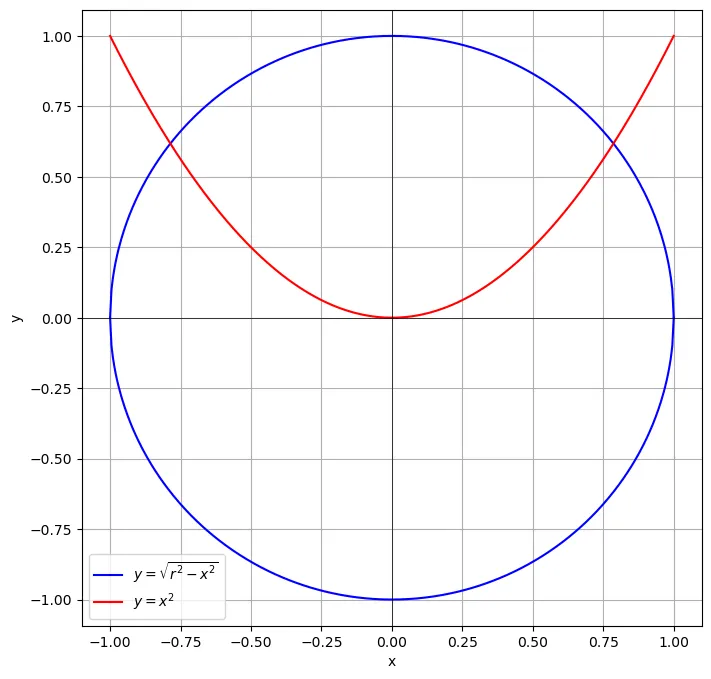
Consider the set of all points on a plane. The relation defined by the equation of a circle, $x^2 + y^2 = r^2$, includes all points $(x, y)$ that satisfy this equation. This relation is not a function because, for most values of $x$, there are two possible values of $y$ that satisfy the equation, one positive and one negative (except for the points where $x = \pm r$, where there is only one value of $y$).

In contrast, a function would allow each $x$ to be associated with exactly one $y$. For instance, the square function $y = x^2$ is a function because each value of $x$ corresponds to exactly one value of $y$.

In the figure we have defined a circle and a quadratic function, clearly we see that a function can never have two $y$ value for one $x$, while this is possible for the circle.

ExampleLet A be the set 1, 2, 3, 4

Let A be the set {1,2,3,4}. Which ordered pairs are in the relation $R=\{(a,b)\mid a$ divides $b\}?$

Solution: Because $(a,b)$ is in R if and only if $a$ and $b$ are positive integers not exceeding 4 such that $a$ divides $b$,we see that

$$R=\{(1,1),(1,2),(1,3),(1,4),(2,2),(2,4),(3,3),(4,4)\}.$$

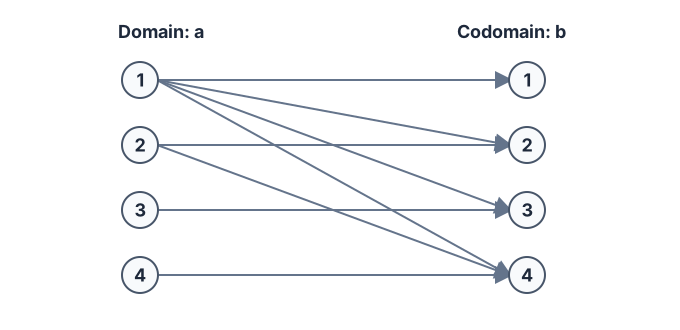
This relation also differs from function, since for member of $a$, it is possible to map to multiple members in $b$.

DefinitionFunctional Relations

A relation $R$ is said to be functional if each element of its domain has exactly one $R$-relative; a functional relation is also called a function. If $R$ is a functional relation then for each element $a$ of its domain we denote the unique $R$-relative of $a$ by $R(a).$

This leads us to the next axiom of NBG theory.

AxiomReplacement Axiom

For every functional relation $R$, if the domain of $R$ is a set then the range of $R$ is also a set.

Mapping, Composition, and Inverse

In naive set theory and function in part 1 of the book, we gave a rough definitions to mappings. With class, we can make it more concrete.

DefinitionMappings

A mapping is an ordered pair $((A,B),R)$ where $A$ and $B$ are sets and $R$ is a functional relation between $A$ and $B$ such that Dom $R=A.$ If $f= ( ( A, B) , R)$ is a mapping we say that $f$ is a mapping from $A$ to $B;$ we call $A$ the domain of $f,B$ the codomain of $f$ and $R$ the graph of $f$. If $f$ is a mapping with domain $A$ and codomain $B$ we often write $f:A\to B.$ If $a$ is any element of the set $A$ then the set $R^{\to}(\{a\})$ consists of a single element of $B$ which we denote by $f(a);$ we call it the image of $a\textbf{ under }f$ or the value of $f\textbf{ at }a.$

It is clear from the definition of the term "mapping" that in order to describe a mapping $f$ we must give the domain $A$ and codomain $B$ of $f$ and also, for each element $a$ of the domain we must describe the unique element $b_a$ of the codomain such that $(a,b_a)$ belongs to the graph of $f$, i.e. we must describe for each element $a$ of $A$ its image under $f$ in $B.$

Let $f= ( ( A, B) , R)$ be a mapping from $A$ to $B$. For each subset $X$ of $A$ we denote the subset $R^{\to}(X)$ of $B$ by $f^{\to}(X);$ in particular, if $a$ is any element of $A$ we have $f^{\to}(\{a\})=\{f(a)\}.$ For each subset $Y$ of $B$ we denote the subset $R^{\leftarrow }( Y)$ of $A$ by $f^{\leftarrow }( Y) .$

Let $f=((A,B),R)$ be a mapping from $A$ to $B$, and let $A_1$ be a subset of $A$. Then the restriction of $f$ to $A_1$ is the mapping

$$f\mid A_1= \left((A_1,B),R\cap(A_1\times B)\right).$$

Earlier, we discussed composition and inverse of function. Now that we have known that function is a kind of relation, can we compose or inverse all other relations? Naturally the answer is yes.

DefinitionSurjective Mappings

Let $f= ( ( A, B) , R)$ be a mapping. Then $f$ is said to be surjective or to be a surjection if we have Range $R$ $= B,$i.e. if every element of $B$ is the image under $f$ of at least one element of $A.$

Next, $f$ is injective if the inverse relation $R^{-1}$ is functional. Equivalently, each element of the range of $R$ is the image under $f$ of exactly one element of $A$. In symbols, whenever $f(a_1)=f(a_2)$ for $a_1,a_2\in A$, we have $a_1=a_2$.

The mapping $f$ is said to be bijective or to be a bijection if it is both injective and surjective. If $A$ and $B$ are sets we say that $A\textbf{is}$ equipotent to $B$ or that $A\textbf{is equinumerous with }B$ if there exists a bijective mapping from $A$ to $B.$

Let $f=((A,B),R)$ be a mapping. Then $((B,A),R^{-1})$ is a mapping if and only if $f$ is bijective; in this case we write $((B,A),R^{-1})=f^{-1}$ and call $f^{-1}$ the inverse mapping of $f.$ Clearly $f^{-1}$ is a bijection from $B$ to $A$ with inverse $f.$

Here are some examples of special mappings.

ExampleA function f: A B is surjective if for every element y in B, there is...

A function $f: A \to B$ is surjective if for every element $y$ in $B$, there is at least one element $x$ in $A$ such that $f(x) = y$. For instance, let $A = \{1, 2, 3\}$ and $B = \{a, b\}$. Define $f$ by $f(1) = a$, $f(2) = a$, and $f(3) = b$. This function is surjective because every element of $B$ is the image of at least one element of $A$.

ExampleA function f: A B is injective if no two different elements in A map...

A function $f: A \to B$ is injective if no two different elements in $A$ map to the same element in $B$. For example, let $A = \{1, 2, 3\}$ and $B = \{a, b, c, d\}$. Define $f$ by $f(1) = a$, $f(2) = b$, and $f(3) = c$. This function is injective because each element of $A$ maps to a unique element of $B$.

ExampleA function f: A B is bijective if it is both injective and surjective

A function $f: A \to B$ is bijective if it is both injective and surjective. For instance, let $A = \{1, 2, 3\}$ and $B = \{a, b, c\}$. Define $f$ by $f(1) = a$, $f(2) = b$, and $f(3) = c$. This function is bijective, making $A$ and $B$ equinumerous.

ExampleIf f is a bijective function from A to B, then the inverse f^-1 is a...

If $f$ is a bijective function from $A$ to $B$, then the inverse $f^{-1}$ is a function from $B$ to $A$ that reverses the mapping of $f$. Using the bijective function $f$ from the previous example, we define $f^{-1}$ by $f^{-1}(a) = 1$, $f^{-1}(b) = 2$, and $f^{-1}(c) = 3$.

DefinitionComposition of Relations

If $R$ and $S$ are relations, the composition of $R$ and $S$ is the relation $S\circ R$ given by

$$S\circ R=\{(x,z):(\exists y)(((x,y)\in R)\wedge((y,z)\in S))\}.$$

If $R$ is a relation between $A$ and $B$ and $S$ is a relation between $B$ and $C$ then clearly $S\circ R$ is a relation between $A$ and $C$, and we have $\operatorname{Dom}\left(S\circ R\right)\subseteq\operatorname{Dom}R$ and Range $(S\circ R)\subseteq\operatorname{Range}S.$

The idea of composition also works for mappings.

DefinitionComposition of Mappings

Let $f= ( ( A, B) , R)$ and $g= ( ( B, C) , S)$ be mappings. Then clearly $((A,C),S\circ R)$ is also a mapping, which we denote by $g\circ f$ and call the composition or composed mapping of $f$ and $g$. For each element $a$ of $A$ we have $( g\circ f) ( a) = g( f( a) ).$

RemarkComposition Notation

The other equivalent definition is that Let $R$ be a relation from a set $A$ to a set $B$ and S a relation from $B$ to a set $C$. The $composite$ of $R$ and S is the relation consisting of ordered pairs $(a,c)$, where $a\in A, c\in C$ , and for which there exists an element $b\in B$ such that $( a, b) \in R$ and $( b, c) \in S.$ We denote the composite of $R$ and $S$ by $S\circ R.$

Similarly, we can define inverse relation.

DefinitionRelations Between Classes

If $A$ and $B$ are classes then a relation between $A\textbf{ and }B$ is a subclass of $A\times B$, i.e. a relation $R$ such that Dom $R\subseteq A$ and Range $R\subseteq B.$ A relation on a class $A$ is a subclass of $A\times A.$

If $R$ is a relation, the inverse of $R$ is the relation $R^{-1}$ given by

$$R^{-1}=\{(x,y):(y,x)\in R\}.$$

If $R$ is a relation between $A$ and $B$ then $R^{-1}$ is a relation between $B$ and $A;$ clearly Dom $R^{-1}=\operatorname{Range}R$ and Range $R^{-1}=\operatorname{Dom}R.$

Let $R$ be a relation, $A$ any class. Then the image of $A\textbf{ under }R$ is the class consisting of all $R$-relatives of all members of $A.$ We denote this class by $R^{\to}(A).$ Thus

$$R^{\to}(A)=\{y:(\exists x)((x\in A)\land((x,y)\in R))\}.$$

Again let $R$ be a relation and $\ker B$ be any class. Then the inverse image of $B$ under $R$ is the class $( R^{- 1}) ^{\to }( B) ,$ which we write $R^{\leftarrow}( B) .$ Thus

$$\begin{aligned}R^{\leftarrow}(B)=\{x:(\exists y)((y\in B)\land((x,y)\in R))\}.\end{aligned}$$

With functional relation and mapping, we can define a more specific relation, which very special and practical.

DefinitionThe Diagonal Relation

Let $A$ be any set; let $D_A=\{x:(\exists a)((a\in A)\land(x=(a,a)))\}$ (we call $D_A$ the diagonal of $A\times A).$ Then $D_A$ is a functional relation between $A$ and $A$ with domain $A.$ The mapping $I_A=((A,A),D_A)$ from $A$ to $A$ is called the identity mapping of $A.$ Clearly we have $I_{A}(a)=a$ for each element $a$ of $A.$

ExampleThe identity mapping IA for a set A is a function that maps every...

The identity mapping $I_A$ for a set $A$ is a function that maps every element to itself. Here are some examples of identity mappings on various sets:

• Let $B = \{x \in \mathbb{R} \mid -1 \leq x \leq 1\}$. The identity mapping on $B$ is $I_B : B \to B$ where $I_B(x) = x$ for all $x \in B$.

• Let $C = \{\text{apple}, \text{banana}, \text{cherry}\}$. The identity mapping on $C$ is $I_C : C \to C$ where $I_C(\text{fruit}) = \text{fruit}$ for each fruit in set $C$.

• Let $D = \mathbb{Z}$. The identity mapping on $D$ is $I_D : \mathbb{Z} \to \mathbb{Z}$ where $I_D(n) = n$ for all $n \in \mathbb{Z}$.

The diagonal for each of these sets would be as follows:

• The diagonal of $B$, $D_B$, would be the set of all ordered pairs $(x, x)$ such that $x \in B$.

• The diagonal of $C$, $D_C$, would be the set $\{(\text{apple}, \text{apple}), (\text{banana}, \text{banana}), (\text{cherry}, \text{cherry})\}$.

• The diagonal of $D$, $D_D$, would be the set of all ordered pairs $(n, n)$ such that $n \in \mathbb{Z}$.

In all these cases, the identity mapping illustrates the concept of a function where the input is the same as the output for each element of the set.

Families of Sets

In part 1, we discussed sequence. Sequence is defined (see definition def_sequence) by a relation between index and a mathematical expression related to the index, and commonly the index $i$ has $i\in \mathbb{N}$. Sequence is actually a special family of set.

DefinitionFamilies of Elements

Let $I$ and $A$ be classes, and $F$ is a functional relation between $I$ and $A$. Then $F$ is sometimes called a family of elements of $A$ indexed by $I$ (or with $I\textbf{ as index class})$ and we write $(F(i))_{i\in I}$ instead of $F$. In particular, if $E$ is a set then a family of elements of $\mathbf{P}(E)$ is called a family of subsets of $E$ indexed by $I.$ If $F$ is such a family and we write $X_i=F(i)$ for each element $i$ in $I$ then we denote the family $F$ by$\left ( X_i\right ) _{i\in I}.$

If $X$ is a set of subsets of a set $E$ then the diagonal $D_X$ is a family of subsets of $E$ which may sometimes be denoted by $(x)_{x\in X}.$

Let $F= ( X_{i}) _{i\in I}$ be a family of subsets of a set $E.$ We define the union of the family to be

$$\bigcup_{i\in I}X_i=\{x:(\exists i)((i\in I)\land(x\in X_i))\}.$$

Thus $x$ belongs to the union of the family $(X_i)_{i\in I}$ if and only if it belongs to at least one of the sets $X_i$ with $i$ in $I.$ Of course if $X$ is a set of subsets of $E$ the union of the corresponding family $D_X$ coincides with the union of the set $X$ as previously defined: $\bigcup_{x\in X}x=\bigcup X.$

Again let $(X_i)_{i\in I}$ be a family of subsets of a set $E.$ The intersection of this family is defined to be

$$\bigcap_{i\in I}X_i=\{x:(x\in E)\land(\forall i)((i\in I)\Longrightarrow(x\in X_i))\}.$$

So $x$ belongs to the intersection of the family $(X_i)_{i\in I}$ if and only if it belongs to all the sets $X_i$ with $i$ in $I.$

We notice that if $I$ is empty then we have $\bigcap_{i\in I}X_i=E.$ If X i a non-empty set of subsets of $E$ the intersection of the corresponding family $D_X$ coincides with the intersection of the set $X$ as previously defined${: }\bigcap _{x\in X}x= \bigcap X.$

ExampleConsider the set E and a family of its subsets (Xi)i in I, where I =...

Consider the set $E$ and a family of its subsets $(X_i)_{i \in I}$, where $I = \{1, 2, 3\}$ and

• $X_1 = \{a, b\}$

• $X_2 = \{b, c\}$

• $X_3 = \{a, c, d\}$

The union of the family $(X_i)_{i \in I}$ is the set of elements that are in at least one of the sets $X_i$:

$$\bigcup_{i \in I} X_i = X_1 \cup X_2 \cup X_3 = \{a, b, c, d\}$$

The intersection of the family $(X_i)_{i \in I}$ is the set of elements that are in every one of the sets $X_i$:

$$\bigcap_{i \in I} X_i = X_1 \cap X_2 \cap X_3 = \emptyset$$

DefinitionSequences as Functions

Let $E$ be a set. A sequence in $E$ is a function from the set of natural numbers $\mathbb{N}$ to $E$. The sequence can be represented as a family of sets $(x_i)_{i \in \mathbb{N}}$, where each $x_i$ is an element of $E$, and $i$ is the index representing the position of the element in the sequence.

The $n$-th term of the sequence is denoted by $x_n$, and the sequence itself can be written as $(x_n)_{n=1}^{\infty}$, which is the family of elements of $E$ indexed by $\mathbb{N}$.

Let $(X_i)_{i\in I}$ be a family of sets with index set $I.$ Let $X=\bigcup_{i\in I}X_i.$ Then the product of the family $(X_i)_{i\in I}$ is the set

$$\prod_{i\in I}X_i=\{f:(f\in\operatorname{Map}(I,X))\wedge(\forall i)((i\in I)\Longrightarrow(f(i)\in X_i))\}.$$

If we write $f(i)=x_i$ for each index $i$ in $I$, it is sometimes helpful to denote the element $f$ of $\prod_{i\in I}X_i$ by $\prod_{i\in I}x_i$.

For each index $j$ in $I$ we define a mapping $\pi_j$ from $\prod_{i\in I}X_i$ to $X_j$ by setting

$$\pi_j(f)=f(j)\quad\text{for every }f\in\prod_{i\in I}X_i.$$

The mapping $\pi_j$ is called the $j$ -th projection mapping from $\prod_{i\in I}X_i.$

ExampleConsider two sets X1 = a, b and X2 = 1, 2

Consider two sets $X_1 = \{a, b\}$ and $X_2 = \{1, 2\}$. The index set is $I = \{1, 2\}$. The product of the family of sets $(X_i)_{i \in I}$, which is $X_1 \times X_2$, consists of all ordered pairs where the first element is from $X_1$ and the second is from $X_2$. Thus, the product is:

$$\prod_{i \in I} X_i = X_1 \times X_2 = \{(a, 1), (a, 2), (b, 1), (b, 2)\}$$

Each ordered pair represents a function $f$ mapping $I$ to the union of $X_1$ and $X_2$. For instance, one such function corresponding to the ordered pair $(a, 1)$ is defined by:

$$f(1) = a, \quad f(2) = 1$$

Projection mappings $\pi_j$ from $\prod_{i \in I} X_i$ to $X_j$ are defined for each index $j \in I$ by setting:

$$\pi_1(f) = f(1), \quad \pi_2(f) = f(2)$$

Hence, for our function $f$, the projections are:

$$\pi_1(f) = a, \quad \pi_2(f) = 1$$

Family of Sets is related to another axiom of NBG set theory.

AxiomCartesian Product Axiom

Let $(E_i)_{i\in I}$ be a family of nonempty sets indexed by a set $I$. Then the product $\prod_{i\in I}E_i$ is non-empty.

We can also define choice function of class.

DefinitionChoice Functions

Let $(E_i)_{i\in I}$ be a family of non-empty sets. By a choice function for this family we mean a mapping $f$ from $I$ to $\bigcup_{i\in I}E_i$ such that for every index $i$ in $I$ we have $f(i)\in E_i;$ thus a choice function is an element of the product $\prod_{i\in I}E_i.$ If we have $E_i\cap E_j=\emptyset$ for every pair of distinct elements $i, j$ of $I$ we say that the family $( E_i) _{i\in I}$ is $pairwise$ $disjoint)$ then the range of a choice function for $(E_i)_{i\in I}$ is a subset of $\bigcup_{i\in I}E_i$ which contains exactly one element from each set of the family. Such a set is called a selection set for the (pairwise disjoint) family $(E_i)_{i\in I}.$

Thus the Axiom of Choice asserts that for every family of non-empty sets there exists a choice function and so for every pairwise disjoint family of non-empty sets there exists a selection set.

ExampleConsider the family of non-empty, pairwise disjoint sets

Consider the family of non-empty, pairwise disjoint sets:

$$$$$$\begin{aligned} E_1 &= \{1, 2\}, \\ E_2 &= \{3, 4\}, \\ E_3 &= \{5, 6\}, \end{aligned}$$$$$$

with the index set $I = \{1, 2, 3\}$.

A choice function $f$ for this family might be defined as:

$$$$$$\begin{aligned} f(1) &= 1, \\ f(2) &= 4, \\ f(3) &= 5. \end{aligned}$$$$$$

This function $f$ chooses one element from each set $E_i$, making the selection set for this family $\{ f(1), f(2), f(3) \} = \{1, 4, 5\}$.

Reflexivity, Symmetry, and Transitivity

With basic relation we have defined, we can now look into some special relations with some specific properties. These properties are important, since these property will be used to further classify relations for us. All special relations could be related to the diagonal of the sets or classes involved in that specific relation.

The first special relation is actually already covered in the diagonal of class, which is the idea of reflexivity, meaning a relation from an object to itself.

DefinitionReflexive Relations

Let $R$ be a relation on a set $X$. The relation $R$ is said to be reflexive if $D_X \subseteq R$, where $D_X = \{(x, x) \mid x \in X\}$. That is, for every element $x$ in $X$, the pair $(x, x)$ belongs to $R$.

ExampleConsider the following relations on the set 1, 2, 3, 4

Consider the following relations on the set $\{1, 2, 3, 4\}$:

• $R_1 = \{(1, 1), (1, 2), (2, 1), (2, 2), (3, 4), (4, 1), (4, 4)\}$

• $R_2 = \{(1, 1), (1, 2), (2, 1)\}$

• $R_3 = \{(1, 1), (1, 2), (1, 4), (2, 1), (2, 2), (3, 3), (4, 1), (4, 4)\}$

• $R_4 = \{(2, 1), (3, 1), (3, 2), (4, 1), (4, 2), (4, 3)\}$

• $R_5 = \{(1, 1), (1, 2), (1, 3), (1, 4), (2, 2), (2, 3), (2, 4), (3, 3), (3, 4), (4, 4)\}$

• $R_6 = \{(3, 4)\}$

Which of these relations are reflexive?

Solution: The relations $R_3$ and $R_5$ are reflexive because they both contain all pairs of the form $(a, a)$, namely, $(1, 1), (2, 2), (3, 3),$ and $(4, 4)$. The other relations are not reflexive because they do not contain all of these ordered pairs. In particular, $R_1, R_2, R_4,$ and $R_6$ are not reflexive because $(3, 3)$ is not in any of these relations.

And as a complement of Reflexivity, we can define Irreflexivity

DefinitionIrreflexive Relations

A relation $R$ on a set $X$ is called irreflexive if $D_X \cap R = \emptyset$, i.e., no pair of the form $(x, x)$ belongs to $R$ for any $x$ in $X$.

Now we discuss symmetry of relation.

DefinitionSymmetric Relations

A relation $R$ on a set $X$ is symmetric if for every $x, y$ in $X$, if $(x, y) \in R$ then $(y, x)$ is also in $R$, i.e., $R = R^{-1}$

We can also define the complement of this kind of relation.

DefinitionAsymmetric Relations

Let $R$ be a relation on a set $X$. The relation $R$ is said to be asymmetric if for any $x, y$ in $X$, whenever $(x, y) \in R$, then $(y, x) \notin R$. This implies that no pair can be in both $R$ and $R^{-1}$ unless $x = y$, which is not permitted for asymmetric relations, thus $R \cap R^{-1} = \emptyset$, i.e. $R \neq R^{-1}$, .

There is also a type of relation called antisymmetric relation.

DefinitionAntisymmetric Relations

A relation $R$ on a set $X$ is antisymmetric if for all $x, y$ in $X$, if $(x, y) \in R$ and $(y, x) \in R$, then $x = y$. That is, $R \cap R^{-1} \subseteq D_X$.

Some may confused by these similar terms. Below are the clarification and some examples.

• A relation $R$ on a set $X$ is symmetric if for any $x, y \in X$, whenever $(x, y)$ is in $R$, then $(y, x)$ is also in $R$. Symmetry implies a mutual relationship.

• A relation $R$ is asymmetric if for any $x, y \in X$, whenever $(x, y)$ is in $R$, $(y, x)$ is not in $R$. Asymmetry denotes a one-way relationship.

• A relation $R$ is antisymmetric if for any $x, y \in X$, whenever both $(x, y)$ and $(y, x)$ are in $R$, it must be that $x = y$. Antisymmetry allows for a hierarchical ordering.

Let's explore these properties through examples:

ExampleThe relation 'is a sibling of' is symmetric

The relation "is a sibling of" is symmetric. If Tom is a sibling of Jerry, then Jerry is a sibling of Tom.

ExampleThe 'less than' relation on the real numbers is asymmetric

The "less than" relation on the real numbers is asymmetric. If $3 < 4$, then it is not the case that $4 < 3$.

ExampleThe 'divides' relation for integers is antisymmetric

The "divides" relation for integers is antisymmetric. For example, $6$ divides $12$, and $12$ does not divide $6$. But we can have 6 divides 6 itself.

Exercises

ExerciseDetermine whether each of the following is a set or a class in NBG set...

Determine whether each of the following is a set or a class in NBG set theory, and explain why.

1. The collection of all sets that do not contain themselves.

2. The set of all natural numbers.

3. The class of all ordinal numbers.

SolutionBelow are the solutions The collection of all sets that do not contain...

Below are the solutions.

1. The collection of all sets that do not contain themselves is a proper class. This is because any attempt to consider it as a set leads to Russell's paradox, thus it cannot be a set within any consistent set theory including NBG.

2. The set of all natural numbers is a set. It is well-defined and does not lead to any paradoxes within NBG set theory. Furthermore, it is an element of the class of all sets.

3. The class of all ordinal numbers is a proper class because it is too large to be a set. If it were a set, it would lead to contradictions similar to those arising from considering the "set of all sets."

ExerciseRussel's Paradox is fixed by introducing more strict set axioms to the...

Russel's Paradox is fixed by introducing more strict set axioms to the set theory. In NBG theory, a proper class is defined as a top-level class that cannot be subclass of any other classes or sets, and this is the key to avoid the paradox in naive set theory. Explain in details that how this concept avoids the case in Russel's Paradox.

SolutionWith the introduction of the concept of classes, we can discuss...

With the introduction of the concept of classes, we can discuss collections that are too large to be considered as sets, such as the "class of all sets." Therefore, the set described by Russell's Paradox, denoted by $R$, is no longer considered a legitimate set but rather a "proper class." This means that we refrain from discussing $R$ as a set, thereby avoiding the paradox because proper classes are not subject to the operations and axioms that constrain sets. As a result, the axiomatic system does not permit the formation of sets that would lead to Russell's Paradox.

ExerciseLet A, B, C be classes such that A B, B C, C A

Let $A,B,C$ be classes such that $A\subseteq B,B\subseteq C$, $C\subseteq A.$ Prove that $A=B=C.$

ExerciseLet A, B, C be classes such that A B, B C

Let $A,B,C$ be classes such that $A\subset B,B\subset C.$ Prove that $A\subset C.$

Below are exercises for binary relation.

Representation of Relations

In last section. we discussed binary relation and their properties. This section focuses on ways of representation. Symbolic language is accurate and not prone to make misunderstanding, yet it is not quite easy to understand to human minds. Therefore, we need straightforward ways to visualize them and assure the accuracy in the same time.

Representation By Matrix

The first commonly used method is matrix. A relation between finite sets can be represented using a zero-one matrix. Suppose that $R$ is a relation from $A=\{a_1,a_2,\ldots,a_m\}$ to $B=\{b_1,b_2,\ldots,b_n\}.$ (Here the elements of the sets $A$ and $B$ have been listed in a particular, but arbitrary, order. Furthermore, when $A=B$ we use the same ordering for $A$ and $B.)$ The relation $R$ can be represented by the matrix $\mathbf{M}_R=[m_{ij}]$, where

$$m_{ij}=\left\{\begin{matrix}1\text{ if}(a_i,b_j)\in R,\\0\text{ if}(a_i,b_j)\notin R.\end{matrix}\right.$$

ExampleConsider the binary relation R on the set X = 1, 2, 3 defined by the...

Consider the binary relation $R$ on the set $X = \{1, 2, 3\}$ defined by the pairs $R = \{(1, 2), (2, 3), (3, 1)\}$. We can represent $R$ as a matrix $M$ where the entry $m_{ij}$ is 1 if $(i, j) \in R$ and 0 otherwise. Thus, the matrix $M$ representing $R$ is given by:

$$M = \begin{bmatrix} 0 & 1 & 0 \\ 0 & 0 & 1 \\ 1 & 0 & 0 \end{bmatrix}$$

This matrix shows that there is a relation from 1 to 2, 2 to 3, and 3 to 1, as indicated by the ones in the matrix.

What about some other special relations? Here are more examples.

Reflexive Relations in Matrix

We defined reflexivity through the diagonal of a relation matrix. A relation on a set is reflexive if and only if every diagonal entry $m_{ii}$ is $1$. The off-diagonal entries may be chosen independently, so a reflexive relation need not be the identity relation.

ExampleA reflexive relation on a set X = 1, 2, 3 requires that every element...

A reflexive relation on a set $X = \{1, 2, 3\}$ requires that every element is related to itself. Thus, for the relation $R$ to be reflexive, it must include the pairs $R = \{(1, 1), (2, 2), (3, 3)\}$ at minimum. The matrix $M$ representing such a reflexive relation $R$ is given by:

$$M = \begin{bmatrix} 1 & a & b \\ c & 1 & d \\ e & f & 1 \end{bmatrix}$$

Here, the diagonal elements of the matrix are all set to 1, reflecting the reflexive property that each element is related to itself. This diagonal structure is reminiscent of an identity matrix, where all diagonal elements are 1, and all off-diagonal elements are 0. In the context of relations, the presence of 1s on the diagonal is crucial for reflexivity. However, the values of $a, b, c, d, e,$ and $f$ (the off-diagonal elements) do not influence the reflexivity of the relation and can be either 0 or 1. This highlights that while the matrix representing a reflexive relation must have 1s along its diagonal, it does not necessarily need to be an identity matrix.

Symmetric/Antisymmetric/Asymmetry Relation in Matrix

For a symmetric relation, $(a,b)\in R$ if and only if $(b,a)\in R$. In its matrix, this means $m_{ij}=m_{ji}$, or equivalently $M=M^T$. Symmetry does not require the diagonal entries to be $1$; that additional condition belongs to reflexivity.

ExampleA relation R on a set X = 1, 2, 3 is symmetric if for any two elements...

A relation $R$ on a set $X = \{1, 2, 3\}$ is symmetric if for any two elements $a$ and $b$ in $X$, whenever $(a, b) \in R$, then $(b, a)$ is also in $R$. Consider the symmetric relation $R$ defined by the pairs $R = \{(1, 1), (3, 3), (1, 2), (2, 1)\}$. The matrix $M$ representing this symmetric relation $R$ is given by:

$$M = \begin{bmatrix} 1 & 1 & 0 \\ 1 & 0 & 0 \\ 0 & 0 & 1 \end{bmatrix}$$

In this matrix, the entries are symmetric about the main diagonal. The presence of $1$ at positions $(1,2)$ and $(2,1)$ illustrates the symmetric nature of the relation, as both $(1,2)$ and $(2,1)$ are included in $R$.

A reflexive relation, on the other hand, requires that each element be related to itself, leading to $1$s along the main diagonal of its matrix. In the example above, the relation is not reflexive because it does not contain $(2, 2)$.

Although both reflexive and symmetric properties concern the main diagonal, they describe different aspects of a relation:

• Reflexivity is about individual elements being self-connected, evidenced by $1$s on the diagonal.

• Symmetry involves pairs of elements and requires that if an element $a$ is related to an element $b$, then $b$ must also be related to $a$, leading to a mirrored symmetry across the diagonal.

A relation can be both reflexive and symmetric but does not need to be one to be the other. For instance, a purely symmetric relation need not include self-pairs like $(1, 1)$ unless it is also intended to be reflexive.

An antisymmetric relation on a set $X$ involves a specific condition: for any two distinct elements $\alpha$ and $b$ in $X$,if both $(a,b)$ and $(b,a)$ are in the relation $R$, then $\alpha$ must be equal to $b$. This means that if $a\neq$ $b$,it cannot be the case that both $(a,b)$ and $(b,a)$ are in $R$.In terms of matrix representation:

ExampleConsider the set X = 1, 2, 3 and define the relation R on X by the...

Consider the set $X = \{1, 2, 3\}$ and define the relation $R$ on $X$ by the pairs $R = \{(1, 2), (2, 3), (3, 3)\}$. This relation is antisymmetric, which we can observe through its matrix representation. The matrix $M$ representing the relation $R$ is given by:

$$M = \begin{bmatrix} 0 & 1 & 0 \\ 0 & 0 & 1 \\ 0 & 0 & 1 \end{bmatrix}$$

In this matrix, note the following:

• The entry $m_{12} = 1$ (relation from 1 to 2), and $m_{21} = 0$ (no relation from 2 to 1), satisfying the antisymmetric condition.

• Similarly, $m_{23} = 1$ and $m_{32} = 0$.

• The diagonal entry $m_{33} = 1$ does not violate antisymmetry as self-relations do not affect antisymmetry.

Antisymmetric relations allow entries on the main diagonal (self-relations) but restrict how elements can relate symmetrically off the diagonal, ensuring that if one direction is permitted, the opposite is not unless they are the same element.

An asymmetric relation is a stronger form of an antisymmetric relation. A relation $R$ on a set $X$ is asymmetric if, for any elements $a$ and $b$ in $X$,whenever $(a,b)$ is in $R$, then $(b,a)$ cannot be in $R$. This implies that if one direction between two different elements is allowed, the opposite direction is strictly forbidden, making it impossible for both $(a,b)$ and $(b,a)$ to exist in $R$ for any $a\neq b.$

ExampleConsider the set X = 1, 2, 3 and define an asymmetric relation R on X...

Consider the set $X = \{1, 2, 3\}$ and define an asymmetric relation $R$ on $X$ by including the pairs $R = \{(1, 2), (2, 3)\}$. This relation is asymmetric as it does not contain both $(a, b)$ and $(b, a)$ for any $a$ and $b$ in $X$. The matrix $M$ representing this relation $R$ is given by:

$$M = \begin{bmatrix} 0 & 1 & 0 \\ 0 & 0 & 1 \\ 0 & 0 & 0 \end{bmatrix}$$

In this matrix: - The entry $m_{12} = 1$ and $m_{21} = 0$, supporting the asymmetric nature by the absence of the reverse relation. - The entry $m_{23} = 1$ and $m_{32} = 0$, further demonstrating asymmetry.

This matrix shows no reciprocal relations between different elements, which is a defining characteristic of asymmetric relations. Note that self-relations (diagonal entries) are not present in this matrix, aligning with the strict definition of asymmetry which typically excludes self-relations as well.

Operation of Relation Matrix

We can find intersection or union of two relations easily by examining their matrices. This could be done by comparing each element with the same index one by one.

ExampleLet A = bmatrix 0 & 1 & 0 0 & 0 & 1 0 & 0 & 0 bmatrix and B = bmatrix...

Let $A = \begin{bmatrix} 0 & 1 & 0 \\ 0 & 0 & 1 \\ 0 & 0 & 0 \end{bmatrix}$ and $B = \begin{bmatrix} 1 & 1 & 0 \\ 0 & 0 & 0 \\ 1 & 0 & 0 \end{bmatrix}$ be two relations.

The union $A \cup B$ is:

$$A \cup B = \begin{bmatrix} 1 & 1 & 0 \\ 0 & 0 & 1 \\ 1 & 0 & 0 \end{bmatrix}$$

The intersection $A \cap B$ is:

$$A \cap B = \begin{bmatrix} 0 & 1 & 0 \\ 0 & 0 & 0 \\ 0 & 0 & 0 \end{bmatrix}$$

Matrix is also possible to represent composition of relations. For these relations, in particular, suppose that $R$ is a relation from $A$ to $B$ and $S$ is a relation from $B$ to $C$. Suppose that $A$, $B$, and $C$ have $m$, $n$, and $p$ elements, respectively. Let the zero-one matrices for $S \circ R$, $R$, and $S$ be $M_{S \circ R} = [t_{ij}]$, $M_R = [r_{ij}]$, and $M_S = [s_{ij}]$, respectively (these matrices have sizes $m \times p$, $m \times n$, and $n \times p$, respectively). The ordered pair $(a_i, c_j)$ belongs to $S \circ R$ if and only if there is an element $b_k$ such that $(a_i, b_k)$ belongs to $R$ and $(b_k, c_j)$ belongs to $S$. It follows that $t_{ij} = 1$ if and only if $r_{ik} = s_{kj} = 1$ for some $k$. From the definition of the Boolean product, this means that

$$M_{S \circ R} = M_R \otimes M_S.$$

ExampleMR = 1 & 0 & 1 1 & 1 & 0 0 & 0 & 0 and MS =

$$M_R = \begin{bmatrix} 1 & 0 & 1 \\ 1 & 1 & 0 \\ 0 & 0 & 0 \\ \end{bmatrix} \quad \text{and} \quad M_S = \begin{bmatrix} 0 & 1 & 0 \\ 0 & 0 & 1 \\ 1 & 0 & 1 \\ \end{bmatrix}.$$

SolutionThe matrix for S R is obtained by performing the Boolean product of MR...

The matrix for $S \otimes R$ is obtained by performing the Boolean product of $M_R$ and $M_S$. This operation is similar to matrix multiplication, except that addition is replaced by the logical OR operation, and multiplication is replaced by the logical AND operation. The result is a matrix that represents the composition of the two relations:

$$M_{S \circ R} = M_R \otimes M_S = \begin{bmatrix} 1 & 1 & 1 \\ 0 & 1 & 1 \\ 0 & 0 & 0 \\ \end{bmatrix}.$$

Each entry in $M_{S \circ R}$ is computed by taking the logical OR of the ANDs of the corresponding row from $M_R$ and the column from $M_S$.

Examplewhere the matrix representing R is MR = 0 & 1 & 0

where the matrix representing $R$ is

$$M_R = \begin{bmatrix} 0 & 1 & 0 \\ 0 & 1 & 1 \\ 1 & 0 & 0 \\ \end{bmatrix}.$$

SolutionThe matrix for R^2 is found by taking the Boolean product of MR with...

The matrix for $R^2$ is found by taking the Boolean product of $M_R$ with itself. This operation is analogous to squaring a matrix, where we use Boolean algebra for addition and multiplication:

$$M_{R_2} = M_{R}^{[2]} = \begin{bmatrix} 0 & 1 & 1 \\ 1 & 1 & 1 \\ 0 & 1 & 0 \\ \end{bmatrix}.$$

The entries of $M_{R_2}$ indicate whether there is a path of length 2 between the nodes represented by the matrix indices in the relation $R$.

Representation By Digraph

The other way to visualize relation is by using Directed Graph, or Digraph.

DefinitionDirected Graphs

A digraph or directed graph is an ordered pair $G = (V, A)$ comprising:

• A non-empty set $V$, whose elements are called vertices or nodes.

• A set $A$ of ordered pairs of vertices, called arcs, directed edges, arrows, or directed lines.

The directed edge $(x, y) \in A$ is said to point from the vertex $x$ to the vertex $y$. Unlike in an undirected graph, the edges in a digraph have a direction associated with them, indicated by the ordering of the vertices in the pair.

We will discuss further on graph in graph theory, now we just need to know that we will use it to visualize relation. A directed graph can be used to represent a binary relation between a set of elements. Here is an example.

ExampleLet set A = a, b, c, B = a, d, the relation R=(a, a), (a, d), (b, a),...

Let set $A = \{a,b,c\}, B = \{a,d\}$, the relation

$$R=\{(a,a),(a,d), (b,a),(c,a),(c,d)\}$$

could be represented by the following graph.

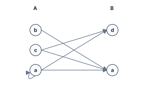
Using Digraph is a very intuitive approach to visualize relation. In the graph, we use the element in the domain and codomain of the relation as vertex, and the relations are represented using the edges, which are also ordered pairs.

Using a graph is also easy to determine special patterns of relations such as reflexivity, symmetry, etc.

ExampleConsider the relation defined from set A=a, b, c to itself, R = (a,...

Consider the relation defined from set $A=\{a,b,c\}$ to itself, $R = \{(a,a),(b,b),(c,c),(b,a)\}$. This relation could be visualized by the following graph, which is reflexive.

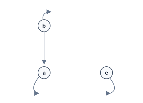
We see that each object has a loop for a reflexive relation.

ExampleConsider the relation defined from set A=a, b, c to itself, R1 = (a,...

Consider the relation defined from set $A=\{a,b,c\}$ to itself, $R_1 = \{(a,b),(b,a)(a,c),(c,a)\}$, and $R_2=\{(a,a),(b,b)(c,c),(a,b),(b,c) \}$. This relation could be visualized by the following graphs.

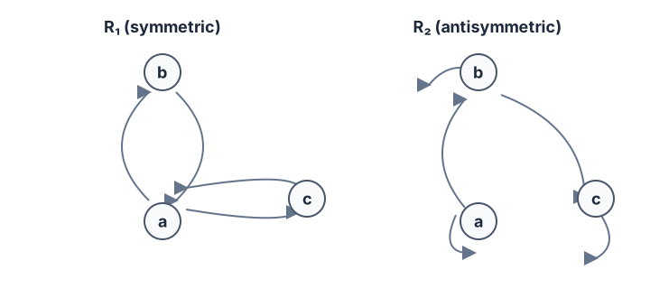
$R_1$ is symmetric because every edge between distinct objects has a matching edge in the opposite direction. $R_2$ is antisymmetric because the only pairs that occur in both directions are self-loops, although it may contain one-way edges between distinct objects.

For the cases of transitivity, it's also quite clear in the following example.

ExampleStill consider the same set A and the relation R1 = (a, b), (b, c),...

Still consider the same set $A$ and the relation $R_1 = \{(a,b), (b,c), (a,c)\}, R_2 = \{(a,a), (a,b),(b,b)\}$.

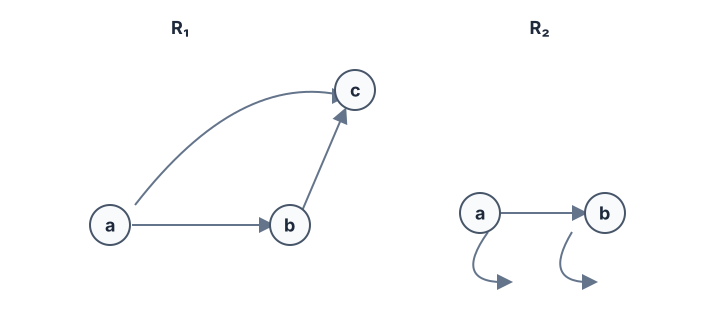
Both $R_1$ and $R_2$ are transitive. For $R_2$, transitivity follows in particular from the reflexive loops on $a$ and $b$. A relation that is reflexive, symmetric, and transitive is an equivalence relation, which we discuss next.

Exercises

ExerciseList the ordered pairs in the relations on 1, 2, 3, 4 corresponding to...

List the ordered pairs in the relations on $\{1, 2, 3, 4\}$ corresponding to these matrices (where the rows and columns correspond to the integers listed in increasing order).

$$\text{a)} \begin{bmatrix} 1 & 1 & 0 & 1 \\ 1 & 0 & 1 & 0 \\ 0 & 1 & 1 & 1 \\ 1 & 0 & 1 & 1 \\ \end{bmatrix} \text{b)} \begin{bmatrix} 1 & 1 & 1 & 0 \\ 0 & 1 & 0 & 0 \\ 0 & 0 & 1 & 1 \\ 1 & 0 & 0 & 1 \\ \end{bmatrix} \text{c)} \begin{bmatrix} 0 & 1 & 0 & 1 \\ 1 & 0 & 1 & 0 \\ 0 & 1 & 0 & 1 \\ 1 & 0 & 1 & 0 \\ \end{bmatrix}$$

SolutionSince the (1, 1)^th entry is a 1, (1, 1) is in the relation

1. Since the $(1,1)^{th}$ entry is a $1$, $(1,1)$ is in the relation. Since $(1,3)^{th}$ entry is a $0$, $(1,3)$ is not in the relation. Continuing in this manner, we see that the relation contains $(1,1)$, $(1,2)$, $(1,4)$, $(2,1)$, $(2,3)$, $(3,2)$, $(3,3)$, $(3,4)$, $(4,1)$, $(4,3)$, and $(4,4)$.

2. The relation contains $(1,1)$, $(1,2)$, $(1,3)$, $(2,2)$, $(3,3)$, $(3,4)$, $(4,1)$, and $(4,4)$.

3. The relation contains $(1,2)$, $(1,4)$, $(2,1)$, $(2,3)$, $(3,2)$, $(3,4)$, $(4,1)$, and $(4,3)$.

ExerciseRepresent each of these relations on 1, 2, 3, 4 with a matrix (with...

Represent each of these relations on $\{1, 2, 3, 4\}$ with a matrix (with the elements of this set listed in increasing order).

1. $\{(1, 2), (1, 3), (1, 4), (2, 3), (2, 4), (3, 4)\}$

2. $\{(1, 1), (1, 4), (2, 2), (3, 3), (4, 1)\}$

3. $\{(1, 2), (1, 3), (1, 4), (2, 1), (2, 3), (2, 4), (3, 1), (3, 2), (3, 4), (4, 1), (4, 2), (4, 3)\}$

4. $\{(2, 4), (3, 1), (3, 2), (3, 4)\}$

SolutionThe relations corresponding to these matrices (from a to d) are

The relations corresponding to these matrices (from a to d) are:

$$\begin{bmatrix} 0 & 1 & 1 & 1 \\ 0 & 0 & 1 & 1 \\ 0 & 0 & 0 & 1 \\ 0 & 0 & 0 & 0 \end{bmatrix} \begin{bmatrix} 1 & 0 & 0 & 1 \\ 0 & 1 & 0 & 0 \\ 0 & 0 & 1 & 0 \\ 1 & 0 & 0 & 0 \end{bmatrix} \begin{bmatrix} 0 & 1 & 1 & 1 \\ 1 & 0 & 1 & 1 \\ 1 & 1 & 0 & 1 \\ 1 & 1 & 1 & 0 \end{bmatrix} \begin{bmatrix} 0 & 0 & 0 & 0 \\ 0 & 0 & 0 & 1 \\ 1 & 1 & 0 & 1 \\ 0 & 0 & 0 & 0 \end{bmatrix}$$

ExerciseHow many nonzero entries does the matrix representing the relation R...

How many nonzero entries does the matrix representing the relation $R$ on $A = \{1, 2, 3, ..., 1000\}$ consisting of the first 1000 positive integers have if $R$ is

1. $\{(a, b) \mid a \leq b\}$?

2. $\{(a, b) \mid a = b \pm 1\}$?

3. $\{(a, b) \mid a + b = 1000\}$?

4. $\{(a, b) \mid a + b \leq 1001\}$?

5. $\{(a, b) \mid a \neq 0\}$?

SolutionNote that the total number of entries in the matrix is 1000^2 = 1,...

Note that the total number of entries in the matrix is $1000^2 = 1,000,000$.

1. There is a $1$ in the matrix for each pair of distinct positive integers not exceeding $1000$, namely in position $(a, b)$ where $a \leq b$, as well as $1$'s along the diagonal. Thus the answer is the number of subsets of size $2$ from a set of $1000$ elements, plus $1000$, i.e., $C(1000, 2) + 1000 = 499500 + 1000 = 500,500$.

2. There two $1$'s in each row of the matrix except the first and last rows, in which there is one $1$. Therefore the answer is $998 \cdot 2 + 2 = 1998$.

3. There is a $1$ in the matrix at each entry just above and to the left of the "anti-diagonal" (i.e., in positions $(1, 999), (2, 998), ..., (999, 1)$. Therefore the answer is $999$.

4. There is a $1$ in the matrix at each entry on or above (to the left of) the "anti-diagonal." This is the same number of $1$'s as in part (a), so the answer is again $500,500$.

5. The condition is trivially true (since $1 \leq a \leq 1000$), so all $1,000,000$ entries are $1$.

ExerciseDraw the directed graph that represents the relation (a, a), (a, b),...

Draw the directed graph that represents the relation

$$\{(a, a), (a, b), (b, c), (c, b), (c, d), (d, a), (d, b).\}$$

ExerciseLet R be a relation on a set A

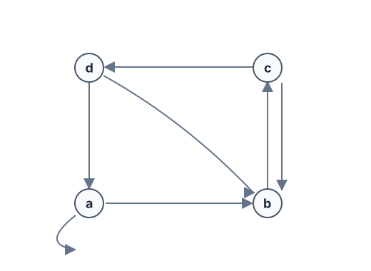
Let $R$ be a relation on a set $A$. Explain how to use the directed graph representing $R$ to obtain the directed graph representing the complementary relation $\overline{R}$.

SolutionFor each pair (a, b) of vertices (including the pairs (a, a) in which...

For each pair $(a, b)$ of vertices (including the pairs $(a, a)$ in which the two vertices are the same), if there is an edge from $a$ to $b$, then erase it, and if there is no edge from $a$ to $b$, put add it in.

ExerciseGiven the directed graphs representing two relations, how can the...

Given the directed graphs representing two relations, how can the directed graph of the union, intersection, symmetric difference, difference, and composition of these relations be found?

SolutionWe assume that the two relations are on the same set

We assume that the two relations are on the same set. For the union, we simply take the union of the directed graphs, i.e., take the directed graph on the same vertices and put in an edge from $i$ to $j$ whenever there is an edge from $i$ to $j$ in either of them. For intersection, we simply take the intersection of the directed graphs, i.e., take the directed graph on the same vertices and put in an edge from $i$ to $j$ whenever there are edges from $i$ to $j$ in both of them. For symmetric difference, we simply take the symmetric difference of the directed graphs, i.e., take the directed graph on the same vertices and put in an edge from $i$ to $j$ whenever there is an edge from $i$ to $j$ in one, but not both, of them. Similarly, to form the difference, we take the difference of the directed graphs, i.e., take the directed graph on the same vertices and put in an edge from $i$ to $j$ whenever there is an edge from $i$ to $j$ in the first but not the second. To form the directed graph for the composition $S \circ R$ of relations $R$ and $S$, we draw a directed graph on the same set of vertices and put in an edge from $i$ to $j$ whenever there is a vertex $k$ such that there is an edge from $i$ to $k$ in $R$, and an edge from $k$ to $j$ in $S$.

Closure of Relations

Section Pending Migration / Draft Placeholder

This section on relation closures (reflexive closure, symmetric closure, and transitive closure via Warshall's algorithm) is an outline placeholder from the original lecture notes, queued for complete exposition and proofs.

Equivalence Relations

In mathematics, an equivalence relation is a special type of binary relation that allows us to group elements of a set into disjoint subsets called equivalence classes. The idea behind equivalence relations is to capture a meaningful notion of "sameness" or "interchangeability" among elements.

Equivalence relations are characterized by three key properties: reflexivity, symmetry, and transitivity. These properties ensure that the relation partitions the set into equivalence classes, each containing elements that are equivalent in some sense.

Equivalence

DefinitionEquivalence Relations

A relation on a set $A$ is called an equivalence relation if it is reflexive, symmetric, and transitive. Two elements $a$ and $b$ that are related by an equivalence relation are called equivalent. The notation $a\sim b$ is often used to denote that $a$ and $b$ are equivalent elements with respect to a particular equivalence relation.

The concept of equivalence relations is a fundamental tool in many branches of mathematics. They allow us to focus on essential characteristics that elements share, abstracting away extraneous details. Some common examples include:

• Equality of numbers

• Congruence modulo $n$ in number theory

• Similarity of triangles in geometry

• Having the same cardinality for sets

Equivalence relations provide a way to decompose a set into a collection of equivalence classes, revealing important structural insights. They are essential for understanding quotient structures, modular arithmetic, and the role of abstraction in mathematical thought.

ExampleLet m be an integer with m > 1

Let $m$ be an integer with $m > 1$. Show that the relation

$$R = \{(a, b) \mid a \equiv b \ (\mathrm{mod} \ m)\}$$

is an equivalence relation on the set of integers.

SolutionRecall from Section 4

Recall from Section 4.1 that $a \equiv b \ (\mathrm{mod} \ m)$ if and only if $m$ divides $a - b$. Note that $a - a = 0$ is divisible by $m$, because $0 = 0 \cdot m$. Hence, $a \equiv a \ (\mathrm{mod} \ m)$, so congruence modulo $m$ is reflexive.

Now suppose that $a \equiv b \ (\mathrm{mod} \ m)$. Then $a - b$ is divisible by $m$, so $a - b = km$, where $k$ is an integer. It follows that $b - a = (-k)m$, so $b \equiv a \ (\mathrm{mod} \ m)$. Hence, congruence modulo $m$ is symmetric.

Next, suppose that $a \equiv b \ (\mathrm{mod} \ m)$ and $b \equiv c \ (\mathrm{mod} \ m)$. Then $m$ divides both $a - b$ and $b - c$. Therefore, there are integers $k$ and $l$ with $a - b = km$ and $b - c = lm$. Adding these two equations shows that $a - c = (a - b) + (b - c) = km + lm = (k + l) m$. Thus, $a \equiv c \ (\mathrm{mod} \ m)$. Therefore, congruence modulo $m$ is transitive.

It follows that congruence modulo $m$ is an equivalence relation.

ExampleLet A be a non-empty set, and define a relation on the power set P(A)...

Let $A$ be a non-empty set, and define a relation $\sim$ on the power set $\mathcal{P}(A)$ (the set of all subsets of $A$) as follows: for any subsets $X, Y \subseteq A$,

$$X \sim Y \iff |X| = |Y|$$

where $|X|$ denotes the cardinality (number of elements) of the set $X$. In other words, two subsets are related by $\sim$ if and only if they have the same number of elements.

SolutionWe can show that the relation defined above is an equivalence relation...

We can show that the relation $\sim$ defined above is an equivalence relation on $\mathcal{P}(A)$:

1. Reflexivity: For any subset $X \subseteq A$, we have $|X| = |X|$, so $X \sim X$.

2. Symmetry: If $X \sim Y$, then $|X| = |Y|$. Since equality of cardinalities is symmetric, we also have $|Y| = |X|$, so $Y \sim X$.

3. Transitivity: If $X \sim Y$ and $Y \sim Z$, then $|X| = |Y|$ and $|Y| = |Z|$. By the transitivity of equality, we have $|X| = |Z|$, so $X \sim Z$.

The equivalence classes under this relation are called cardinality classes. For a subset $X \subseteq A$, its cardinality class $[X]$ consists of all subsets of $A$ that have the same cardinality as $X$:

$$[X] = {Y \subseteq A \mid |Y| = |X|}$$

In other words, the cardinality classes partition $\mathcal{P}(A)$ into disjoint subsets based on the number of elements in each subset. For example, if $A = {1, 2, 3}$, then the cardinality classes are:

• $[\emptyset] = { \emptyset }$ (subsets with 0 elements)

• $[{1}] = {{1}, {2}, {3}}$ (subsets with 1 element)

• $[{1, 2}] = {{1, 2}, {1, 3}, {2, 3}}$ (subsets with 2 elements)

• $[A] = {A}$ (subsets with 3 elements)

This equivalence relation captures the idea that two sets are "equivalent" if they have the same cardinality, regardless of their specific elements. The study of cardinality and the relationships between sets of different sizes is a fundamental aspect of set theory and plays a crucial role in the development of modern mathematics, including the theory of infinite sets and the foundations of mathematics.

ExampleLet R be the relation on the set of real numbers such that xRy if and...

Let $R$ be the relation on the set of real numbers such that $xRy$ if and only if $x$ and $y$ are real numbers that differ by less than 1, that is, $|x - y| < 1$. Show that $R$ is not an equivalence relation.

SolutionR is reflexive because |x - x| = 0 < 1 whenever x in R

$R$ is reflexive because $|x - x| = 0 < 1$ whenever $x \in \mathbb{R}$. $R$ is symmetric, for if $xRy$, where $x$ and $y$ are real numbers, then $|x - y| < 1$, which tells us that $|y - x| = |x - y| < 1$, so that $yRx$. However, $R$ is not an equivalence relation because it is not transitive. Take $x = 2.8$, $y = 1.9$, and $z = 1.1$, so that $|x - y| = |2.8 - 1.9| = 0.9 < 1$, $|y - z| = |1.9 - 1.1| = 0.8 < 1$, but $|x - z| = |2.8 - 1.1| = 1.7 > 1$. That is, $2.8R1.9$, $1.9R1.1$, but not $2.8R1.1$.

Equivalence Classes

We can dig deeper into equivalence by partitioning the set where the relation is built upon with respect to a member of the subset. We call this a Equivalence Class.

DefinitionEquivalence Classes

Let $R$ be an equivalence relation on a set A. The set of all elements that are related to an element $a$ of $A$ is called the $equivalence$ class of $a$. The equivalence class of $a$ with respect to $R$ is denoted by $[a]_R$. When only one relation is under consideration, we can delete the subscript $R$ and write $[a]$ for this equivalence class.

RemarkRepresentatives of Equivalence Classes

In set notation we have

$$[a]_R = \{ (a,s) \in R\}.$$

For some member $e\in [a]_R$, we call $e$ a representative of the equivalence class.

ExampleWhat is the equivalence class of an integer for the equivalence...

What is the equivalence class of an integer for the equivalence relation $a = |b|$?

SolutionSince a = b or a = -b, so [a] = -a, a, which holds for all integer,...

Since $a = b \text{ or } a = -b$, so $[a] = \{-a,a\}$, which holds for all integer, including 0. We have $[3] = \{ -3, 3\}$, etc.

ExampleWhat are the equivalence classes of 0 and 1 for congruence modulo 2?

What are the equivalence classes of 0 and 1 for congruence modulo 2?

SolutionThe equivalence class of 0 contains all integers a such that a == 0 mod 4

The equivalence class of 0 contains all integers $a$ such that $a \equiv 0 \pmod{4}$. The integers in this class are those divisible by 4. Hence, the equivalence class of 0 for this relation is

$$[0] = \{ \ldots, -8, -4, 0, 4, 8, \ldots \}.$$

The equivalence class of 1 contains all the integers $a$ such that $a \equiv 1 \pmod{4}$. The integers in this class are those that have a remainder of 1 when divided by 4. Hence, the equivalence class of 1 for this relation is

$$[1] = \{ \ldots, -7, -3, 1, 5, 9, \ldots \}.$$

This notion actually allows us to further abstract to congruence classes modulo $m$.

DefinitionCongruence Classes Modulo an Integer

Let $m$ be a positive integer. The congruence class of an integer $a$ modulo $m$, denoted by $[a]_m$, is the set of all integers $b$ such that $b \equiv a \ (\mathrm{mod} \ m)$, which means that $m$ divides $b - a$. Formally, the congruence class $[a]_m$ is defined as:

$$[a]_m = \{ b \in \mathbb{Z} \ | \ b \equiv a \ (\mathrm{mod} \ m) \} = \{ b \in \mathbb{Z} \ | \ \exists k \in \mathbb{Z}, \ b = a + km \}.$$

Here are some other examples on equivalence class.

ExampleFind the equivalence class for (1)/(2) under the relation of fraction...

Find the equivalence class for $\frac{1}{2}$ under the relation of fraction simplification.

SolutionThe equivalence class of (1)/(2) consists of all fractions that...

The equivalence class of $\frac{1}{2}$ consists of all fractions that simplify to $\frac{1}{2}$, which includes all rational numbers where the numerator is half the denominator. Hence, the equivalence class is:

$$[1/2] = \left\{ \frac{2}{4}, \frac{3}{6}, \frac{4}{8}, \frac{5}{10}, \ldots \right\}$$

ExampleFind the equivalence class for the string 'cat' under the relation of...

Find the equivalence class for the string "cat" under the relation of having the same length.

SolutionThe equivalence class of the string 'cat' consists of all strings of...

The equivalence class of the string "cat" consists of all strings of length 3. Examples include:

$$[\text{"cat"}] = \{ \text{"dog"}, \text{"pen"}, \text{"sun"}, \text{"mom"}, \ldots \}$$

Congruence Class can be further interpreted by introducing partition of set. Recall (in definition def

) that the partition of a set are a possible combination of mutually disjoint subsets of a set. Suppose we have some set $R$, than we can make form some three-member partition $(P_1\cup P_2\cup P_3) = R$, where $P_1,P_2,P_3,\subseteq R$. Also we have $|R| = |P_1|+|P_2|+|P_3|$. But notice that $P_i\cap P_j, i,j \in\{1,2,3\}$ is $\emptyset$.

Now let's relate this to congruence class.

TheoremEquivalence Classes and Partitions

Let $R$ be an equivalence relation on a set $A$. These statements for elements $a$ and $b$ of $A$ are equivalent:

$(i):aRb\quad(ii):[a]=[b]\quad(iii):[a]\cap[b]\neq\emptyset$

Proof

We first show that (i) implies (ii). Assume that $aRb$. We will prove that $[a] = [b]$ by showing $[a] \subseteq [b]$ and $[b] \subseteq [a]$. Suppose $c \in [a]$, where $c$ is any arbitrary member of $[a]$. Then $aRc$. Because $aRb$ and $R$ is symmetric, we know that $bRa$. Furthermore, because $R$ is transitive and $bRa$ and $aRc$, it follows that $bRc$. Hence, $c \in [b]$. This shows that $[a] \subseteq [b]$, since all elements of $[a]$ is also an element of $[b]$. The proof that $[b] \subseteq [a]$ is similar.

Second, we will show that (ii) implies (iii). Assume that $[a] = [b]$. It follows that $[a] \cap [b] \neq \emptyset$ because $[a]$ is nonempty (because $a \in [a]$ since $R$ is reflexive).

Next, we will show that (iii) implies (i). Suppose that $[a] \cap [b] \neq \emptyset$. Then there is an element $c$ with $c \in [a]$ and $c \in [b]$. In other words, $aRc$ and $bRc$. By the symmetric property, $cRb$. Then by transitivity, because $aRc$ and $cRb$, we have $aRb$.

Because (i) implies (ii), (ii) implies (iii), and (iii) implies (i), the three statements, (i), (ii), and (iii), are equivalent.

Let $R$ be an equivalence relation on a set $A$. The union of the equivalence classes is the whole set $A$, because an element a of $A$ is in its own equivalence class, and distinct classes are disjoint (different elements may belong to the same class). $\bigcup_{a\in A}[a]_R=A.$ This is because from theorem one we have

LemmaDistinct Equivalence Classes Are Disjoint

If $[a]_R \neq [b]_R$, then $[a]_R\cap[b]_R=\emptyset.$

If the intersection were nonempty, the preceding equivalence would force the classes to be equal, contradicting the hypothesis. This is the contrapositive of nonempty intersection implying equal classes.

DefinitionPartition

A partition of $S$ is an indexed family of nonempty subsets $A_i$ such that $A_i\cap A_j=\emptyset$ for distinct indices and

$$\bigcup_{i \in I}A_i = S.$$

ExampleLet A = Z, the set of all integers, and let R be the equivalence...

Let $A = \mathbb{Z}$, the set of all integers, and let $R$ be the equivalence relation of congruence modulo $3$. Determine if the following statements are true:

1. $1R4$

2. $[1] = [4]$

3. $[1] \cap [4] \neq \emptyset$

Solution1R4 is true because 4 == 1 mod 3 [1] = [4] is true because both 1 and...

1. $1R4$ is true because $4 \equiv 1 \mod 3$.

2. $[1] = [4]$ is true because both $1$ and $4$ have the same remainder when divided by $3$, which means they are in the same equivalence class modulo $3$.

3. $[1] \cap [4] \neq \emptyset$ is true because $[1]$ contains $4$ since $4 \equiv 1 \mod 3$, hence $4$ is in both $[1]$ and $[4]$.

As all three statements are true, the statements (i), (ii), and (iii) are equivalent for the given equivalence relation.

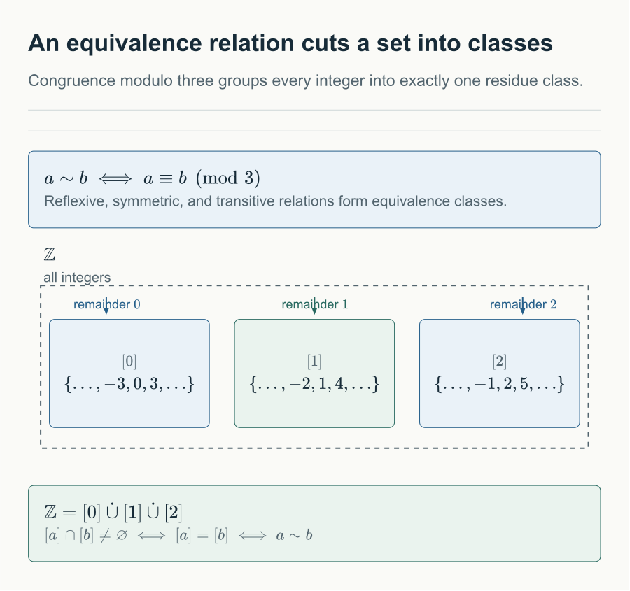
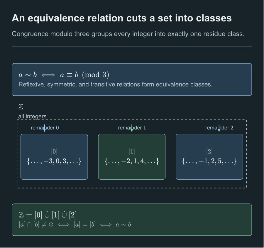
Congruence modulo three partitions all integers into three disjoint equivalence classes.

Exercises

ExerciseDetermine the equivalence class of 2 under the relation of congruence...

Determine the equivalence class of $2$ under the relation of congruence modulo $5$.

SolutionThe equivalence class of 2 modulo 5, denoted [2]5, consists of all...

The equivalence class of $2$ modulo $5$, denoted $[2]_5$, consists of all integers that leave a remainder of $2$ when divided by $5$. This can be expressed as:

$$[2]_5 = \{ \ldots, -8, -3, 2, 7, 12, \ldots \}$$

where each element is of the form $2 + 5k$ for some integer $k$.

ExerciseLet S be the equivalence relation on P(1, 2, 3, 4) defined by X Y if...

Let $S$ be the equivalence relation on $\mathcal{P}(\{1, 2, 3, 4\})$ defined by

$$X \sim Y \text{ if and only if } |X \cup \{2\}| = |Y \cup \{2\}|.$$

Write down the equivalence classes of $S$.

SolutionTo find the equivalence classes of the relation S, we need to analyze...

To find the equivalence classes of the relation $S$, we need to analyze how the sets $X \cup \{2\}$ and $Y \cup \{2\}$ affect the cardinality and thus the equivalence.

Consider the power set $\mathcal{P}(\{1, 2, 3, 4\})$, which includes all subsets of $\{1, 2, 3, 4\}$:

$$\begin{aligned} \mathcal{P}(\{1, 2, 3, 4\}) = & \{\emptyset, \{1\}, \{2\}, \{3\}, \{4\}, \{1, 2\}, \{1, 3\}, \{1, 4\}, \{2, 3\}, \{2, 4\}, \\ & \{3, 4\}, \{1, 2, 3\}, \{1, 2, 4\}, \{1, 3, 4\}, \{2, 3, 4\}, \{1, 2, 3, 4\}\} \end{aligned}$$

We need to group these sets into equivalence classes based on the criterion $|X \cup \{2\}| = |Y \cup \{2\}|$.

1. $\{\emptyset, \{2\}\}$

• $\emptyset \cup \{2\} = \{2\}$, $|\emptyset \cup \{2\}| = 1$

• $\{2\} \cup \{2\} = \{2\}$, $|\{2\} \cup \{2\}| = 1$

2. $\{\{1\}, \{3\}, \{4\}, \{1, 2\}, \{2, 3\}, \{2, 4\}\}$

• $\{1\} \cup \{2\} = \{1, 2\}$, $|\{1\} \cup \{2\}| = 2$

• $\{3\} \cup \{2\} = \{2, 3\}$, $|\{3\} \cup \{2\}| = 2$

• $\{4\} \cup \{2\} = \{2, 4\}$, $|\{4\} \cup \{2\}| = 2$

• $\{1, 2\} \cup \{2\} = \{1, 2\}$, $|\{1, 2\} \cup \{2\}| = 2$

• $\{2, 3\} \cup \{2\} = \{2, 3\}$, $|\{2, 3\} \cup \{2\}| = 2$

• $\{2, 4\} \cup \{2\} = \{2, 4\}$, $|\{2, 4\} \cup \{2\}| = 2$

3. $\{\{1, 3\}, \{1, 4\}, \{3, 4\}, \{1, 2, 3\}, \{1, 2, 4\}, \{2, 3, 4\}\}$

• $\{1, 3\} \cup \{2\} = \{1, 2, 3\}$, $|\{1, 3\} \cup \{2\}| = 3$

• $\{1, 4\} \cup \{2\} = \{1, 2, 4\}$, $|\{1, 4\} \cup \{2\}| = 3$

• $\{3, 4\} \cup \{2\} = \{2, 3, 4\}$, $|\{3, 4\} \cup \{2\}| = 3$

• $\{1, 2, 3\} \cup \{2\} = \{1, 2, 3\}$, $|\{1, 2, 3\} \cup \{2\}| = 3$

• $\{1, 2, 4\} \cup \{2\} = \{1, 2, 4\}$, $|\{1, 2, 4\} \cup \{2\}| = 3$

• $\{2, 3, 4\} \cup \{2\} = \{2, 3, 4\}$, $|\{2, 3, 4\} \cup \{2\}| = 3$

4. $\{\{1, 3, 4\}, \{1, 2, 3, 4\}\}$

• $\{1, 3, 4\} \cup \{2\} = \{1, 2, 3, 4\}$, $|\{1, 3, 4\} \cup \{2\}| = 4$

• $\{1, 2, 3, 4\} \cup \{2\} = \{1, 2, 3, 4\}$, $|\{1, 2, 3, 4\} \cup \{2\}| = 4$

Therefore, the equivalence classes are:

$$\begin{aligned} &\{\emptyset, \{2\}\}, \\ &\{\{1\}, \{3\}, \{4\}, \{1, 2\}, \{2, 3\}, \{2, 4\}\}, \\ &\{\{1, 3\}, \{1, 4\}, \{3, 4\}, \{1, 2, 3\}, \{1, 2, 4\}, \{2, 3, 4\}\}, \\ &\{\{1, 3, 4\}, \{1, 2, 3, 4\}\}. \end{aligned}$$

ExerciseLet A = Z, and define R on A by xRy if and only if x - y is even

Let $A = \mathbb{Z}$, and define $R$ on $A$ by $xRy$ if and only if $x - y$ is even. Determine if the following statements are true for $a = 2$ and $b = 5$:

1. $aRb$

2. $[2] = [5]$

3. $[2] \cap [5] \neq \emptyset$

SolutionaRb is false because 2 - 5 is odd [2] = [5] is false because 2 is in...

1. $aRb$ is false because $2 - 5$ is odd.

2. $[2] = [5]$ is false because $2$ is in the equivalence class of even remainders while $5$ is in the class of odd remainders.

3. $[2] \cap [5] \neq \emptyset$ is false because $[2]$ contains all even numbers and $[5]$ contains all odd numbers, so they have no elements in common.

In this case, statements (i), (ii), and (iii) are not equivalent because the relation $R$ is not defined as congruence modulo some number but rather by the parity of the difference between elements.

No that we can get partition of a set from a equivalence relation, can we inverse this process? That is, define a equivalence relation with some given set partitions? The answer is yes.

To see this, assume that $\{A_i \mid i \in I\}$ is a partition on $S$. Let $R$ be the relation on $S$ consisting of the pairs $(x, y)$, where $x$ and $y$ belong to the same subset $A_i$, in the partition. To show that $R$ is an equivalence relation we must show that $R$ is reflexive, symmetric, and transitive.

We see that $(a, a) \in R$ for every $a \in S$, because $a$ is in the same subset of $S$ as itself. Hence, $R$ is reflexive. If $(a, b) \in R$, then $b$ and $a$ are in the same subset of $S$ in the partition, so that $(b, a) \in R$ as well. Hence, $R$ is symmetric. If $(a, b) \in R$ and $(b, c) \in R$, then $a$ and $b$ are in the same subset $X$ of $S$ in the partition, and $b$ and $c$ are in the same subset $Y$ of $S$ of the partition. Because the subsets of $S$ in the partition are disjoint and $b$ belongs to $X$ and $Y$, it follows that $X = Y$. Consequently, $a$ and $c$ belong to the same subset of $S$ in the partition, so $(a, c) \in R$. Thus, $R$ is transitive.

It follows that $R$ is an equivalence relation. The equivalence classes of $R$ consist of subsets of $S$ containing related elements, and by the definition of $R$, these are the subsets of $S$ in the partition. The theorem summarizes the connections we have established between equivalence relations and partitions.

TheoremEquivalence Classes Form a Partition

Let $R$ be an equivalence relation on a set $S$. Then the equivalence classes of $R$ form a partition of $S$. Conversely, given a partition $\{A_i \mid i \in I\}$ of the set $S$, there is an equivalence relation $R$ that has the sets $A_i, i \in I$, as its equivalence classes.

Proof

Reflexivity puts each element into its own nonempty class. The preceding lemma makes distinct classes disjoint, and their union is all of $S$, proving a partition. Conversely define $xRy$ when $x,y$ belong to the same partition block. Every element belongs to a block, proving reflexivity, and the definition is symmetric. If $x,y$ share a block and $y,z$ share another, their common element $y$ forces those blocks equal, proving transitivity. For $x\in A_i$, exactly the elements of $A_i$ are related to $x$, so $[x]_R=A_i$. This also proves the two constructions undo each other.

ExampleFor example, consider the set S = 1, 2, 3, 4, 5, 6

For example, consider the set $S = \{1, 2, 3, 4, 5, 6\}$.

One possible equivalence relation $R$ on $S$ is "congruence modulo 3". This relation partitions $S$ into the equivalence classes $[1] = \{1, 4\}$, $[2] = \{2, 5\}$, and $[3] = \{3, 6\}$.

Conversely, consider a partition of $S$ into subsets $A_1 = \{1, 2\}$, $A_2 = \{3, 4\}$, and $A_3 = \{5, 6\}$. The equivalence relation $R$ induced by this partition is such that two numbers are related if and only if they are in the same subset $A_i$.

Order Relations

Another important family is formed by order relations, including partial, total, and well orders. We begin with the most general notion, the partial order, and then specialize it.

Partial, Total, and Well Ordering

DefinitionPartial Orders and Posets

A relation $R$ on a set S is called a partial ordering or partial order if it is reflexive, antisymmetric, and transitive. A set $S$ together with a partial ordering $R$ is called a partial ordered set, or poset, and is denoted by $(S,R)$. Members of S are called elements of the poset.

RemarkNotation for Partial Orders

The reason why partial order relation has a specific notation for poset is because that order relation is usually defined on the same set(for the domain and codomain). For equivalence relation, however, we see more relation between different sets.

The most common partial order relation is "greater than or equal to", "is subset to", and "divides".

ExampleShow that the greater than or equal to relation >= is a partial...

Show that the greater than or equal to relation $\geq$ is a partial ordering on the set of integers.

Solution: Because $a \geq a$ for every integer $a$, $\geq$ is reflexive. If $a \geq b$ and $b \geq a$, then $a = b$. Hence, $\geq$ is antisymmetric. Finally, $\geq$ is transitive because $a \geq b$ and $b \geq c$ imply that $a \geq c$. It follows that $\geq$ is a partial ordering on the set of integers and $(\mathbb{Z}, \geq)$ is a poset.

ExampleThe divisibility relation | is a partial ordering on the set of...

The divisibility relation $|$ is a partial ordering on the set of positive integers, because it is reflexive, antisymmetric, and transitive, as was shown in Section 9.1. We see that $(\mathbb{Z}^+, |)$ is a poset.

ExampleShow that the inclusion relation is a partial ordering on the power...

Show that the inclusion relation $\subseteq$ is a partial ordering on the power set of a set $S$.

Solution: Because $A \subseteq A$ whenever $A$ is a subset of $S$, $\subseteq$ is reflexive. It is antisymmetric because $A \subseteq B$ and $B \subseteq A$ imply that $A = B$. Finally, $\subseteq$ is transitive, because $A \subseteq B$ and $B \subseteq C$ imply that $A \subseteq C$. Hence, $\subseteq$ is a partial ordering on $P(S)$, and $(P(S), \subseteq)$ is a poset.

For convenience of representation, we need a symbol to define the operator for an arbitrary partial ordering.

NotationPartial-Order Notation

$\preccurlyeq$ is used to define any arbitrary partial order relation $a \preccurlyeq b$ on set $S$. Alternatively, we also have $a \prec b$ to denote that $a\preccurlyeq b$ but $a \neq b$.

With this, we can define comparability of the relation. This helps us to distinguish different types of special partial orderings.

DefinitionComparable Elements

The elements $a$ and $b$ of a poset (S, $\preccurlyeq)$ are called comparable if either $a\preccurlyeq b$ or $b\preccurlyeq a$. When $a$ and $b$ are elements of S such that neither $a\preccurlyeq b$ nor $b\preccurlyeq a,a$ and $b$ are called incomparable.

ExampleIn the poset ( Z^+, | ), are 3 and 9 comparable?

In the poset $(\mathbb{Z}^+ ,\mid)$, are 3 and 9 comparable? Also consider 4 and 5.

Solution3 and 9 are obviously comparable, since even though 9 not| 3, we still...

3 and 9 are obviously comparable, since even though $9 \nmid 3$, we still have $3 \mid 9$. So 3 and 9 are comparable. While $4\nmid 5$ and $5\nmid 4$, so they are not comparable.

We see that for divisibility, there are cases that the relation is not comparable among the elements that are involved here. Actually this is why we call it partial order, because there are cases that things cannot be compared or cannot build relation. If we can have a very special partial ordering on $S$ that is comparable for every member of the set, we call it a total ordering or total order relation.

DefinitionTotal Orders

If $(S, \preccurlyeq)$ is a poset and every two elements of $S$ are comparable, $S$ is called a totally ordered or linearly ordered set, and $\preccurlyeq$ is called a total order or a linear order. A totally ordered set is also called a chain.

Total ordering is also very quite familiar to us, actually, the $\leq$ relation we just mentioned is also a total order relation, and so as $\geq$.

Here are some other examples.

ExampleThe set of words in a dictionary with the alphabetical order is a...

The set of words in a dictionary with the alphabetical order is a totally ordered set because any two words can be compared based on lexicographic order.

ExampleThe set of points on a line with a defined direction is a totally...

The set of points on a line with a defined direction is a totally ordered set, where any two points can be compared based on their position relative to each other along the line.

So we know that total orderings are special partial orderings. Now, can we manage to find a kind of special relation with respect to total ordering? The answer is yes, and we have actually known this relation, as it is the foundation of the principal of mathematical induction (theorem principle/induc).

DefinitionWell-Ordered Sets

The poset $(S, \preccurlyeq)$ is a well-ordered set if $\preccurlyeq$ is total ordering and every nonempty subset of $S$ has a least element.

Here are some example of well-ordering.

ExampleThe set of natural numbers N with the usual order <= is not only a...

The set of natural numbers $\mathbb{N}$ with the usual order $\leq$ is not only a totally ordered set but also a well-ordered set because every non-empty subset of $\mathbb{N}$ has a smallest element.

CounterexampleA total order that is not a well-order

Let $S=\{1/n:n\in\mathbb{N},\ n\geq 1\}$. The usual order $\leq$ totally orders $S$, but does not well-order it: the nonempty subset $S$ itself has no least element. For every $1/n\in S$, the smaller element $1/(n+1)$ also belongs to $S$. Well-ordering of $\mathbb{N}$ guarantees least elements of nonempty subsets, not greatest elements.

ExampleThe set of positive integers up to 100, 1, 2, , 100, is well-ordered...

The set of positive integers up to 100, $\{1, 2, \ldots, 100\}$, is well-ordered by the usual $\leq$ relation. Any non-empty subset has a minimum element since it is a finite subset of the well-ordered set $\mathbb{N}$.

Well ordering secures that each step we made with mathematical induction is correct, since the least element allows us to define a solid base case, so that the rest of the statement could be proved one by one by applying our hypothesis, so that the inductive step could be proven. This could be encapsulated by the following theorem.

TheoremWell-Ordered Induction

Suppose that $S$ is a well-ordered set. Then $P(x)$ is true for all $x \in S$, if

Inductive Step: For every $y \in S$, if $P(x)$ is true for all $x \in S$ with $x < y$, then $P(y)$ is true.

Proof

Suppose it is not the case that $P(x)$ is true for all $x \in S$. Then there is an element $y \in S$ such that $P(y)$ is false. Consequently, the set $A = \{ x \in S \mid P(x) \text{ is false} \}$ is nonempty. Because $S$ is well-ordered, $A$ has a least element $a$. By the choice of $a$ as a least element of $A$, we know that $P(x)$ is true for all $x \in S$ with $x < a$. This implies by the inductive step $P(a)$ is true. This contradiction shows that $P(x)$ must be true for all $x \in S$.

RemarkThe Basis Step in Well-Ordered Induction

We do not need a basis step in a proof using the principle of well-ordered induction because if $x_0$ is the least element of a well-ordered set, the inductive step tells us that $P(x_0)$ is true. This follows because there are no elements $x \in S$ with $x < x_0$, so we know (using a vacuous proof) that $P(x)$ is true for all $x \in S$ with $x < x_0$.

Lexicographic Order

In a dictionary, all words are ordered in alphabetical order by the first letter that is different from the other previous words. For example, we have this array of strings in alphabetical order: $\text{"a"}, \text{"abnormal"}, \text{"acknowledge"}, \text{"acquire"},\ldots$. We can conceptualize this ordering in mathematics with a partial order relation, calling it lexicographic order.

The concept of lexicographic ordering can be extended beyond strings and applied to the Cartesian product of two posets. We formalize this concept as follows:

DefinitionLexicographic Ordering

Given two posets $(A_1, \preccurlyeq_1)$ and $(A_2, \preccurlyeq_2)$, the lexicographic ordering $\preccurlyeq$ on $A_1 \times A_2$ compares first coordinates, and compares second coordinates only when the first coordinates are equal. Its strict part is

$$(a_1,a_2)\prec(b_1,b_2)\quad\Longleftrightarrow\quad a_1\prec_1 b_1\ \text{or}\ (a_1=b_1\ \text{and}\ a_2\prec_2 b_2).$$

We achieve a partial ordering $\preccurlyeq$ by combining this lexicographic ordering with equality. Here is how we verify it.

Proof

For reflexivity, every pair $(a_1,a_2)$ is related to itself because $a_1=a_1$ and $a_2\preccurlyeq_2 a_2$.

For antisymmetry, suppose both $(a_1,a_2)\preccurlyeq(b_1,b_2)$ and $(b_1,b_2)\preccurlyeq(a_1,a_2)$. If $a_1\neq b_1$, the strict first-coordinate alternatives would point in opposite directions, which is impossible. Hence $a_1=b_1$. The definition then reduces to $a_2\preccurlyeq_2 b_2$ and $b_2\preccurlyeq_2 a_2$, so $a_2=b_2$ by antisymmetry of $\preccurlyeq_2$.

For transitivity, if the first coordinates are strictly ordered, transitivity of $\preccurlyeq_1$ gives the required first-coordinate comparison. If the first coordinates are equal, the comparison is decided by the second coordinates, where transitivity of $\preccurlyeq_2$ applies. Thus the lexicographic relation is a partial order. It is total when both component orders are total.

ExampleConsider two posets, (A1, <= 1) where A1 = 1, 2 with the usual less...

Consider two posets, $(A_1, \leq_1)$ where $A_1 = \{1, 2\}$ with the usual less than or equal relation, and $(A_2, \leq_2)$ where $A_2 = \{a, b\}$ with $a \leq_2 b$. The lexicographic order $\leq$ on $A_1 \times A_2$ is given as follows:

For any two elements $(a_1, a_2), (b_1, b_2) \in A_1 \times A_2$, we say that $(a_1, a_2) \leq (b_1, b_2)$ if:

1. $a_1 <_1 b_1$, or

2. $a_1 = b_1$ and $a_2 \leq_2 b_2$.

For example, $(1, a) \leq (2, a)$ because $1 <_1 2$, and $(2, a) \leq (2, b)$ because $2 = 2$ and $a \leq_2 b$. Thus, the pair $(1, a)$ is considered less than $(2, b)$ in the lexicographic ordering because the first element of the first pair (1) is less than the first element of the second pair (2), even though we do not compare the second elements in this case.

Hasse Diagram

Section Pending Migration / Draft Placeholder

This subsection on Hasse diagram construction and poset visualization is an outline placeholder from the original lecture notes.

Maximal and Minimal Elements

Section Pending Migration / Draft Placeholder

This subsection covering maximal, minimal, greatest, and least elements in partially ordered sets is queued for complete definitions and examples.

Lattices

Section Pending Migration / Draft Placeholder

This subsection covering lattice properties (meets, joins, and distributive lattices) is queued for authoring.

Topological Sorting

Section Pending Migration / Draft Placeholder

This subsection on topological sorting of finite posets and DAG scheduling algorithms is queued for authoring.

Exercises

The following exercises are on lexicographic ordering.

ExerciseDo some tricks to the result of the proof in definition lexord to make...

Do some tricks to the result of the proof in definition lexord to make it a well order relation.

SolutionThis could be solved without a second thought that we can make A1, A2...

This could be solved without a second thought that we can make $A_1,A_2$ any sets with smallest element, such as $\Z_{1}$, all integers greater than or equal 1.

ExerciseLet R be a binary relation on Z defined by xRy if and only if x < y or...

Let $R$ be a binary relation on $\mathbb{Z}$ defined by

$$xRy \text{ if and only if } x < y \text{ or } x \equiv y \pmod{2}.$$

Is $R$ reflexive? Is $R$ symmetric? Is $R$ antisymmetric? Is $R$ transitive?

Fully justify each answer.

SolutionLet's analyze the properties of the relation R

Let's analyze the properties of the relation $R$.

• Reflexive: A relation $R$ on a set $A$ is reflexive if every element is related to itself, i.e., $aRa$ for all $a \in A$.

  For any integer $x \in \mathbb{Z}$, we have $x \equiv x \pmod{2}$. Hence, $xRx$ holds for all $x \in \mathbb{Z}$.

  Therefore, $R$ is reflexive.

• Symmetric: A relation $R$ on a set $A$ is symmetric if $aRb$ implies $bRa$ for all $a, b \in A$.

  Consider the pair $(2, 3)$. We have $2R3$ because $2 < 3$. However, $3 \not R 2$ because $3 > 2$ and $3 \not\equiv 2 \pmod{2}$.

  Therefore, $R$ is not symmetric.

• Antisymmetric: A relation $R$ on a set $A$ is antisymmetric if $aRb$ and $bRa$ imply $a = b$ for all $a, b \in A$.

  Consider the pair $(2, 4)$. We have $2R4$ because $2 < 4$, and $4R2$ because $4 \equiv 2 \pmod{2}$. However, $2 \neq 4$.

  Therefore, $R$ is not antisymmetric.

• Transitive: A relation $R$ on a set $A$ is transitive if $aRb$ and $bRc$ imply $aRc$ for all $a, b, c \in A$.

  Consider the elements $2$, $3$, and $1$. We have $2R3$ because $2 < 3$, and $3R1$ because $3 \equiv 1 \pmod{2}$. However, $2 \not R 1$ because $2 \not< 1$ and $2 \not\equiv 1 \pmod{2}$.

  Therefore, $R$ is not transitive.

ExerciseExplain why the conjunction of a partial order relation and an...

Explain why the conjunction of a partial order relation and an equivalence relation leads to the previous result.

SolutionA partial order relation is a binary relation that is reflexive,...

A partial order relation is a binary relation that is reflexive, antisymmetric, and transitive. An equivalence relation is a binary relation that is reflexive, symmetric, and transitive.

When we combine a partial order relation with an equivalence relation, the resulting relation can still be reflexive because both component relations are reflexive. However, the antisymmetry of the partial order can conflict with the symmetry of the equivalence relation, leading to a relation that is neither antisymmetric nor symmetric. Furthermore, the transitivity of the partial order might not hold if the conditions of the equivalence relation introduce exceptions, which can break the transitivity in specific cases.

In this particular example: - The reflexive property is preserved because both conditions $x < y$ and $x \equiv y \pmod{2}$ ensure that $xRx$. - The symmetry is broken because $x < y$ does not imply $y < x$. - The antisymmetry is violated when equivalence modulo 2 ($x \equiv y \pmod{2}$) holds for distinct $x$ and $y$. - The transitivity is disrupted when combining the partial order ($x < y$) with equivalence modulo 2, as seen in the counterexample with $2, 3$, and $1$.

Thus, the combined relation $R$ does not retain all properties of partial orders and equivalence relations.

N-ary Relations

Section Pending Migration / Draft Placeholder

This section on $n$-ary relations and relational database models (projections, joins, and keys) is an outline placeholder from the original lecture notes, queued for complete exposition.

Searching algorithms

Searching is the task of locating a target $T$ in an array $A$ of length $n$. The cost depends on whether $A$ is ordered.

Searching in an unordered array

If $A$ has no order, the only general method is to inspect $A[1],\ldots,A[n]$ in turn. This is linear search.

Algorithm 1 Linear search

1:procedure LinearSearch($A, T$)

2:for $j \gets 1$ to $n$ do

3:if $A[j] = T$ then

4:return $j$

5:end if

6:end for

7:return $-1$

8:end procedure

In the worst case every entry is read, so the time is $O(n)$. If $T$ sits in the first cell, a single comparison suffices. Computer scientists record that best-case lower bound with $\Omega$ notation, and a matching upper and lower bound with $\Theta$ notation.

NotationOmega notation

$\Omega(g(n))$ is the set of functions that grow at least as fast as $g$: there exist $c>0$ and $n_0$ such that $0 \leq c g(n) \leq f(n)$ for all $n \geq n_0$.

NotationTheta notation

$\Theta(g(n))$ is the set of functions squeezed between two positive multiples of $g$: there exist $c_1,c_2>0$ and $n_0$ such that $0 \leq c_1 g(n) \leq f(n) \leq c_2 g(n)$ for all $n \geq n_0$.

If the target is equally likely to occupy any index, the average number of probes is

$$\bar{p} = \frac{1}{n}\sum_{i=1}^{n} i = \frac{n+1}{2},$$

so linear search has average cost $\Theta(n)$.

Searching in an ordered array

DefinitionOrdered array

An array $A$ is ordered if $A[1]\leq \cdots \leq A[n]$ or $A[1]\geq \cdots \geq A[n]$.

A comparison with $A[i]$ then discards half of the remaining list:

• if $T < A[i]$, then $T$ cannot occur in $A[i],\ldots,A[n]$;
• if $A[i] < T$, then $T$ cannot occur in $A[1],\ldots,A[i]$.

To make the worst case as small as possible, probe near the middle of the current sublist $A[p],\ldots,A[q]$, using $j=\bigl\lfloor(p+q)/2\bigr\rfloor$. That algorithm is binary search.

Algorithm 2 Binary search

1:procedure BinarySearch($A, T$)

2:$p \gets 1$

3:$q \gets n$

4:while $p \leq q$ do

5:$j \gets \bigl\lfloor (p+q)/2 \bigr\rfloor$

6:if $A[j] = T$ then

7:return $j$

8:else if $A[j] < T$ then

9:$p \gets j+1$

10:else

11:$q \gets j-1$

12:end if

13:end while

14:return $-1$

15:end procedure

A visualisation of the comparisons is available at this search demo.

Walkthrough with $n=12$ and $A=(3,5,8,8,9,16,29,41,50,63,64,67)$. If $T=99$, the variables evolve as follows.

$p$	$j$	$q$	$A[j]$	relation	output
1	6	12	16	$A[j]<T$
7	9	12	50	$A[j]<T$
10	11	12	64	$A[j]<T$
12	12	12	67	$A[j]<T$
13		12			$T$ is not in $A$

Write $k=q-p+1$ for the current length, and after an unsuccessful probe at $A[j]$ split into $k_1=j-p$ and $k_2=q-j$. Choosing $j=\lfloor(p+q)/2\rfloor$ makes $k_1$ the smaller half.

TheoremBinary search sublist lengths

On each iteration with $j=\bigl\lfloor(p+q)/2\bigr\rfloor$, the leftover lengths satisfy

$$k_1 = \Bigl\lfloor \frac{k-1}{2} \Bigr\rfloor \leq k_2 = \Bigl\lceil \frac{k-1}{2} \Bigr\rceil \leq \frac{k}{2}.$$

Proof

From $j \leq (q+p)/2 < j+1$, subtract $p$ to get $k_1 \leq (q-p)/2 < k_1+1$, so $k_1=\lfloor(k-1)/2\rfloor$. Then $k_1+k_2=k-1$ forces the displayed bound on $k_2$.

TheoremBinary search termination

Binary search terminates after at most $\lceil \lg n \rceil + 1$ probes.

Proof

Let $w=\lfloor \lg n \rfloor$. After $w$ unsuccessful probes the current length $k$ is at most $n/2^w$. Since $2^w \leq n < 2^{w+1}$, one has $1 \leq n/2^w < 2$, so $k=1$. The next probe inspects that last entry and then either finds $T$ or makes $p>q$.

DefinitionLoop invariant

A loop invariant is an assertion that is true before and after every iteration of a loop.

Assume $T$ occurs at index $i$. The invariant of the first algorithm is: after $k$ iterations, if $T=A[i]$ then $p\leq i \leq q$.

TheoremLoop invariance of binary search

After $k$ iterations, if $T=A[i]$ then $p\leq i\leq q$.

Proof

Induction on $k$. Before the loop, $p=1$ and $q=n$, so the claim holds. Suppose it holds after $w$ iterations, and another iteration computes $j_{\mathrm{new}}=\lfloor(p+q)/2\rfloor$. Then $p\leq j_{\mathrm{new}}\leq q$. If $A[j_{\mathrm{new}}]<T$, the new left endpoint is $j_{\mathrm{new}}+1$; if $A[j_{\mathrm{new}}]>T$, the new right endpoint is $j_{\mathrm{new}}-1$; if they are equal, $p$ and $q$ are unchanged. In every case the surviving interval still contains $i$ whenever $T$ is present.

When the loop stops with $p>q$, there is no index in $[p,q]$, so $T$ is not in $A$. Otherwise it was returned at the probe $j$. That is why binary search is correct, and much cheaper than linear search.

Branching diagrams

DefinitionBranching diagram

A branching diagram for an algorithm is a tree of all sequences of operations the algorithm might perform.

For $n=12$, the first probe is $A[6]$. The two comparison outcomes lead to $A[3]$ or $A[9]$, and so on.

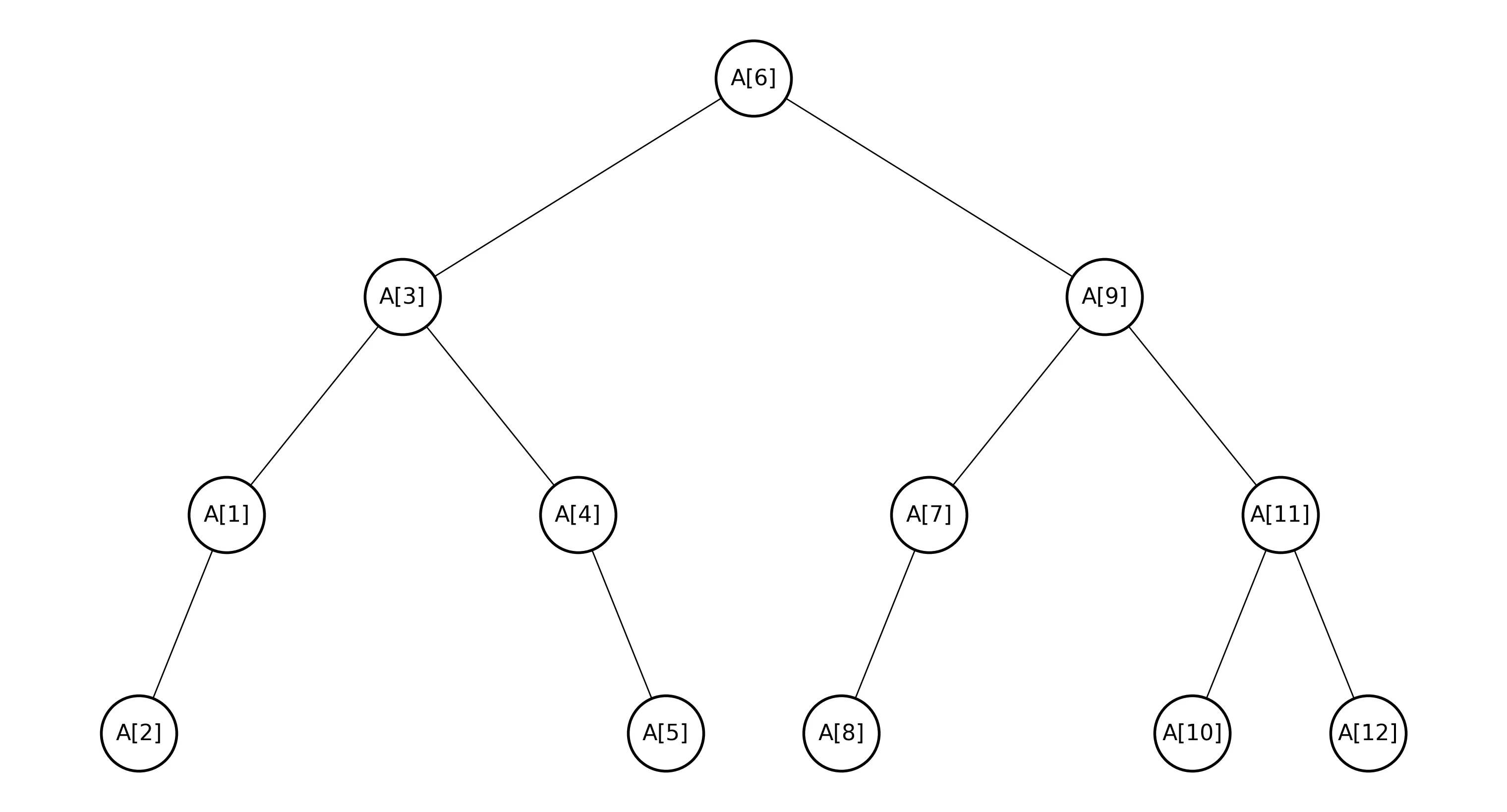
The diagram is a binary tree: it is rooted at the top, every vertex has at most two downward edges, vertices with no downward edge are leaves, and every non-root vertex has exactly one incoming edge from above.

Binary search, version 2

A second version updates the right endpoint by $q \gets j$ rather than $q \gets j-1$, and compares only $A[j]<T$ inside the loop.

Algorithm 3 Binary search, version 2

1:procedure BinarySearch($A, T$)

2:$p \gets 1$

3:$q \gets n$

4:while $p < q$ do

5:$j \gets \bigl\lfloor (p+q)/2 \bigr\rfloor$

6:if $A[j] < T$ then

7:$p \gets j+1$

8:else

9:$q \gets j$

10:end if

11:end while

12:if $A[p] = T$ then

13:return $p$

14:else

15:return $-1$

16:end if

17:end procedure

For the same $T=99$ example the table is shorter by one iteration.

$p$	$j$	$q$	$p<q$	$A[j]$	$A[j]<T$	output
1	6	12	t	16	t
7	9	12	t	50	t
10	11	12	t	64	t
12		12	f			$T$ is not in $A$

The probe $A[j]$ is now the last cell of the left block, not a singleton third block. If $A[j]<T$ one continues in $A[j+1],\ldots,A[q]$; otherwise in $A[p],\ldots,A[j]$. With $j=\lfloor(p+q)/2\rfloor$ the new lengths satisfy $k_2=\lfloor k/2\rfloor \leq k/2 \leq k_1=\lceil k/2\rceil$. So on some iterations the next sublist is more than half as long as the previous one.

Let $L(w)$ be the length still to be searched after $w$ iterations of the while loop.

TheoremLength bounds for version 2

After $w$ iterations,

$$\Bigl\lfloor \frac{n}{2^w} \Bigr\rfloor \leq L(w) \leq \Bigl\lceil \frac{n}{2^w} \Bigr\rceil.$$

Proof

The case $w=0$ is $L(0)=n$. Assume the bound at step $m$. The next length is obtained by taking floor or ceiling of half of $L(m)$. Floor and ceiling are nondecreasing, and for every real $x$ one has $\lfloor\lfloor x\rfloor/2\rfloor=\lfloor x/2\rfloor$ and $\lceil\lceil x\rceil/2\rceil=\lceil x/2\rceil$. Applying these identities with $x=n/2^m$ keeps the same shape of bound at step $m+1$.

TheoremTermination of version 2

After at most $\lceil \lg n \rceil$ comparisons of the form "$A[j]<T$?", and when $p=q$, the current sublist has length $1$.

Lemma

If $x<y$ are real, then $\lceil x\rceil\leq\lceil y\rceil$ and $\lfloor x\rfloor\leq\lfloor y\rfloor$.

The branching diagram of version 2 for $n=12$ is again a binary tree, but every internal vertex has exactly two downward edges: a full binary tree.

TheoremLeaves in a full binary tree

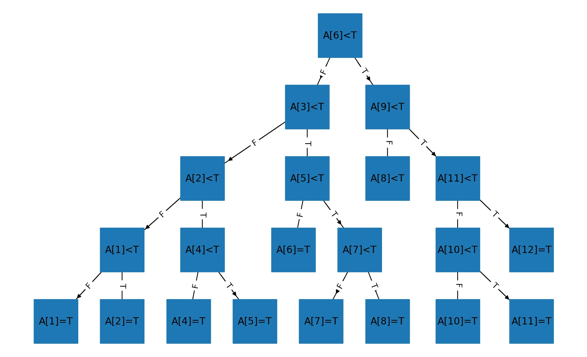
A full binary tree with $m$ internal vertices has $m+1$ leaves.

Proof

Induction on $m$. For $m=1$ the root has two leaf children. Adding one internal vertex converts a leaf into an internal vertex and adds two new leaves, so the leaf count increases by $1$.

Exercises

ExerciseWhere an unsuccessful search would insert

Suppose $T$ is not found by binary search. Where should it be inserted?

1. Is the final $q$ always one less than the final $p$?
2. When is $A[q] < T < A[p]$?
3. If $p=1$ throughout, is $T<A[1]$?
4. If $q=n$ throughout, is $A[n]<T$?

Solution

The final $q$ need not be $p-1$ in every implementation; it depends on how the endpoints move. The inequality $A[q]<T<A[p]$ describes the gap where $T$ would sit in a sorted array. If $p$ never increased then $T<A[1]$; if $q$ never decreased then $A[n]<T$.

ExerciseAverage cost in Theta notation

Consider the best performance of binary search in $\Omega$ notation and the worst performance in $O$ notation. Can the average performance be stated in $\Theta$ notation?

Solution

The best case is a hit at the first midpoint, $\Omega(1)$. The worst case is $O(\log n)$ probes. An average-case $\Theta$ bound would need matching lower and upper estimates under a probability model on the target's index; the usual textbook statement is $O(\log n)$ on average, without a matching $\Theta$ claim, because that model is not unique.

References

1. [1] T. Banakh, “Classical Set Theory: Theory of Sets and Classes,” arXiv:2006.01613, 2026. Version 6, August 15, 2026; NBG sets, classes, and class existence. https://arxiv.org/abs/2006.01613 ↩