Counting and Probability Axioms

In this part, we discuss wider topics on probability and probability distributions. Probability theory is a branch of mathematics that deals with the analysis of random phenomena. The fundamental concept of the theory is the probability measure, a way of assigning a number to each plausible outcome of an event in such a way that the number reflects the event's likelihood of occurring. This mathematical framework allows for the study and modeling of uncertainty and complexity in various fields, ranging from physics and biology to economics and psychology. By providing the tools to make quantitative predictions about the likelihood of certain outcomes, probability theory forms the basis for statistical inference, enabling scientists and statisticians to infer properties about a population given a sample. The origins of probability theory can be traced back to the analysis of games of chance and has since evolved into a vital component of both theoretical and applied mathematics.

Counting Principal

The very first section in this chapter focuses on the basics of counting, which is the foundation of the whole probability theory. In the study of probability, we aim to measure random events, and to do this, we must know their frequency, or rather, how many possible outcomes each event has. Counting method allows us to get the possible number of outcomes in a systematic way.

Principal of Counting

We may start with the most basic counting. Considering tossing a coin, and we make the assumption that this coin is unbiased, meaning that the chance of getting a chance or tail must be exactly $\frac{1}{2}$. In this case, the total possible number of outcome is 2. This conclusion is obviously true and can be obtained by intuition, because we cannot find a third case that the result is neither a head nor a tail, as the event is binary.

Now let's increase the number of trials, how many outcomes can we have when tossing a coin twice? If we use T to denote that the result is a head and F for the tail, like what we have done in Boolean Algebra, we have 4 ways to arrange the possibilities:

$$(T,T), (T,F), (F,T),(F,F).$$

Thus we conclude that we have 4 possible outcomes.

This example lead us to a fundamental theorem in counting.

Theorem

Suppose that two experiments are to be performed. Then if experiment1 can result in any one of $m$ possible outcomes and if, for each outcome of experiment 1, there are $n$ possible outcomes of experiment 2, then together there are $mn$ possible outcomes of the two experiments.

Proof

Partition complete outcomes by their first result. There are $m$ disjoint groups, each containing exactly $n$ outcomes, so finite addition gives $n+\cdots+n=mn$. The second-stage outcomes need not have the same labels in each group; only their counts must agree. No probabilistic independence assumption is required for this counting statement.

Example

A small community consists of 10 women, each of whom has 3 children. If one woman and one of her children are to be chosen as mother and child of the year, how many choices are possible?

Solution

By the product rule of counting, there are $m=10$ outcomes for choosing the woman and $n=3$ outcomes for choosing one of her children. Hence there are $m\times n = 10\times 3 =30$ choices.

But mathematicians hate listing possible cases. Is there a way to describe the relation between the trial of events and number of possible outcomes? Think about the way we treat Boolean variables in the truth table, to get the possible outcomes, we arrange them in all possible ways to get a complete truth table. Just like what we do here, we are making trials twice here for tossing coins, each trial has 2 outcomes, and when we make a truth table, we are generating combinations of Boolean value, and we know that $n$ Boolean variable has $2^n$ ways of arrangement. So we can say that tossing a coin here could be fitted into this relation when $n=2$, and they are actually equivalent in terms of counting the number of outcomes. With this, we can deduce that if we toss the coin for $n$ times, we also have $2^n$ outcomes.

This allows us to generalize theorem Principal of Counting.

Theorem

If $r$ experiments that are to be performed are such that the first one may result in any of $n_1$ possible outcomes; and if, for each of these $n_1$ possible outcomes, there are $n_2$ possible outcomes of the second experiment; and if, for each of the possible outcomes of the first two experiments, there are $n_3$ possible outcomes of the third experiment; and if ..., then there is a total of $\prod_{k=1}^r n_k = n_1 \cdot n_2 \cdots n_r$ possible outcomes of the $r$ experiments.

Proof

Induct on the number of stages $r$. For $r=1$ the count is $n_1$. If the first $r$ stages have $n_1\cdots n_r$ complete prefixes and each prefix has $n_{r+1}$ continuations, the two-stage product rule gives $n_1\cdots n_r n_{r+1}$. This proves every finite number of stages. The empty sequence has one realization, matching the empty product.

This theorem also what we call product rule of counting, which also applicable to probability, which we will discuss in the next section.

Now we introduce another parallel theorem known as addition rule of counting. This is even easier to understand, suppose

Theorem

Suppose that an experiment can be performed in one of $m$ ways or in one of $n$ ways. Where none of the $n$ ways are the same as the $m$ ways, then there are $m+n$ ways to perform it.

This theorem could be proven directly by using set.

Proof

Let $A$ and $B$ be finite sets such that $A \cap B = \emptyset$. By the definition of disjoint sets, no element is in both $A$ and $B$.

Let $a_i$ be an element in $A$ and $b_j$ be an element in $B$, for $i = 1, 2, \ldots, n$ and $j = 1, 2, \ldots, m$. The set $A$ contains exactly $n$ elements and $B$ contains exactly $m$ elements.

The union $A \cup B$ is a set containing all the elements $a_i$ and $b_j$ without any repetition, since $A$ and $B$ are disjoint.

Therefore, the set $A \cup B$ has $n + m$ elements, which proves the theorem.

Example

A student can choose a computer project from one of three lists. The three lists contain 23, 15, and 19 possible projects, respectively. No project is on more than one list. How many possible projects are there to choose from?

Solution

By addition rule, the student can choose a project by selecting a project from the first list, the second list, or the third list. Because no project is on more than one list, by the sum rule there are $23 + 15 + 19 = 57$ ways to choose a project.

Example

How many different license plates can be made if each plate contains a sequence of three uppercase English letters followed by three digits (and no sequences of letters are prohibited, even if they are obscene)?

Solution

To determine the number of different license plates possible, we use the rule of product, also known as the counting principle.

Each of the three positions for the letters can be filled with any of the 26 letters of the English alphabet. Similarly, each of the three positions for the digits can be filled with any of the 10 digits from 0 to 9.

Therefore, the total number of possible license plates is given by:

$$26 \times 26 \times 26 \times 10 \times 10 \times 10 = 26^3 \times 10^3$$

Calculating the powers, we get:

$$26^3 = 26 \times 26 \times 26 = 17576$$$$10^3 = 10 \times 10 \times 10 = 1000$$

Multiplying these together, we find the total number of different license plates that can be made:

$$17576 \times 1000 = 17576000$$

Hence, there are 17,576,000 different possible license plates.

To correctly count the number of ways to do the two tasks, we must subtract the number of ways that are counted twice. This leads us to an important counting rule. Actually, we have already covered this conclusion in set theory.

The Subtraction Rule in set theory is a straightforward concept used when we need to find the number of elements in a set by excluding those that meet certain criteria. It states that if we have a universal set $U$ and a subset $A$ that we wish to exclude, then the number of elements not in $A$ is $|U| - |A|$, where $|S|$ denotes the cardinality of set $S$.

The Principle of Inclusion-Exclusion extends the Subtraction Rule for multiple sets. It corrects the overcounting that occurs when we subtract the cardinalities of overlapping sets from the universal set. For two sets $A$ and $B$, it is given by $|A \cup B| = |A| + |B| - |A \cap B|$.

Theorem

If a task can be done in either $n_1$ ways or $n_2$ ways, then the number of ways to do the task is $n_1+n_2$ minus the number of ways to do the task that are common to the two different ways.

Proof

Decompose the union into the disjoint sets $A\setminus B$, $A\cap B$, and $B\setminus A$. In $|A|+|B|$ the middle set is counted twice and the other two once. Subtracting $|A\cap B|$ leaves each element counted exactly once.

Here are two examples demonstrating these rules.

Example

Suppose a library has 1,000 books, 300 of which are fiction. If we want to know how many books are non-fiction, we can use the Subtraction Rule:

$$\text{Number of non-fiction books} = |U| - |A| = 1,000 - 300 = 700.$$

Example

The proposed data “200 people, 120 liking tea, 150 liking coffee, 50 liking both” are inconsistent: inclusion-exclusion gives $120+150-50=220>200$. The overlap must be at least $120+150-200=70$. If it is $80$, the union is $190$, leaving $10$ who like neither.

We also have division rule of counting, which could be further explained by equivalence class.

Theorem

The rule of division states that there are $n/d$ ways to do a task if it can be done using a procedure that can be carried out in $n$ ways, and for each way $w$, exactly $d$ of the $n$ ways correspond to the way $w$. In a nutshell, the division rule is a common way to ignore "unimportant" differences when counting things.

Proof

The procedure outcomes are partitioned by their final result. If there are $k$ results and each fiber contains exactly $d>0$ outcomes, disjoint addition gives $n=kd$, hence $k=n/d$. Unequal fiber sizes do not permit this division.

This theorem could be further explained by congruence class.

Example

If an $n$-element set is partitioned into classes of size $m>0$, then $n/m$ counts the classes, not arbitrary subsets of the original set. Counting unions of classes would instead give $2^{n/m}$.

Example

If the total degree of a graph is 58, how many edges does it have?

Solution

hen we count the degrees, we count each edge twice, so there are 58/2 = 29 edges.

Pigeonhole Theorem

We also have another useful conclusion on counting called pigeonhole theorem. Suppose we have 8 pigeons and 7 pigeonholes, then there must be one pigeonhole that holds 2 pigeons.

Theorem

If $k$ is a positive integer and $k+1$ or more objects are placed into $k$ boxes, then there is at least one box containing two or more of the objects.

Proof

We prove the pigeonhole principle using a proof by contraposition. Suppose that none of the $k$ boxes contains more than one object. Then the total number of objects would be at most $k$ This is a contradiction, because there are at least $k+1$ objects.

This theorem could also be generalized.

Theorem

If $N$ objects are placed into $k$ boxes, then there is at least one box containing at least $\lceil N/k \rceil$ objects.

Proof

We will prove the statement by contraposition. Let us assume that no box contains $\lceil N/k \rceil$ or more objects. This means each box has at most $\lceil N/k \rceil - 1$ objects. And the number of objects being placed cannot be $N$, so we have the number of object less than $N$ (this is obvious because it can't be greater than $N$).

The total number of objects, under this assumption, can be represented by multiplying the number of boxes by the maximum number of objects each box could contain:

$$k \left( \left\lceil \frac{N}{k} \right\rceil - 1 \right)$$

Using the property that $\lceil x \rceil \leq x + 1$ for any real number $x$, we substitute $\frac{N}{k}$ for $x$ to obtain:

Remark

We get this result in integer function, just in case that you don't remember...

$$\left\lceil \frac{N}{k} \right\rceil \leq \frac{N}{k} + 1$$

Applying this to our previous equation:

$$k \left( \left\lceil \frac{N}{k} \right\rceil - 1 \right) < k \left( \frac{N}{k} + 1 - 1 \right) = N$$

This shows that the total number of objects is less than $N$ under our initial assumption, which is a contradiction since we started with $N$ objects.

Thus, the contrapositive has been proven true: if all boxes have fewer than $\lceil N/k \rceil$ objects, then we do not have $N$ objects. Therefore, by contraposition, the original statement is also true: if $N$ objects are placed into $k$ boxes, there must be at least one box with $\lceil N/k \rceil$ or more objects.

Example

• Among any group of 367 people, there must be at least two with the same birthday, because there are only 366 possible birthdays.

• In any group of 27 English words, there must be at least two that begin with the same letter, because there are 26 letters in the English alphabet.

Example

What is the minimum number of students required in a discrete mathematics class to be sure that at least six will receive the same grade, if there are five possible grades, A, B, C, D, and F?

Proof

The minimum number of students needed to ensure that at least six students receive the same grade can be found using the Pigeonhole Principle. According to this principle, if $N$ objects (in this case, students) are distributed among $k$ categories (in this case, grades), and if $N > k \cdot (m-1)$ where $m$ is the minimum number of objects that we want in at least one category, then at least one category must contain at least $m$ objects.

Here, we want $m = 6$ students to have the same grade and we have $k = 5$ grades. We can apply the formula to find the minimum $N$:

$$N > 5 \cdot (6-1)$$$$N > 25$$

The smallest integer greater than 25 is 26, so at least 26 students are needed to guarantee that at least six will receive the same grade. If we had only 25 students, it could happen that each of the five grades is assigned to exactly five students, which means no grade would have six students. Therefore, 26 is the minimum number of students required to ensure that at least six students will receive the same grade.

Exercises

Exercise

Prove the Generalized Principal of Counting.

Proof

We proceed by mathematical induction on $r$, the number of experiments.

Base Case: For $r = 1$, the theorem trivially holds since there are $n_1$ possible outcomes for the single experiment.

Inductive Step: Assume that the theorem holds for $r = k$, that is, there are $\prod_{i=1}^k n_i$ outcomes for $k$ experiments. Now consider $r = k + 1$ experiments. For the first $k$ experiments, by the inductive hypothesis, we have $\prod_{i=1}^k n_i$ outcomes. For each of these outcomes, the $(k+1)^{th}$ experiment can have $n_{k+1}$ outcomes. Therefore, the total number of outcomes for $k + 1$ experiments is:

$$\left( \prod_{i=1}^k n_i \right) \cdot n_{k+1} = \prod_{i=1}^{k+1} n_i$$

This completes the inductive step and thus the proof.

Exercise

How many functions are there from a set with $m$ elements to a set with $n$ elements?

Solution

A function corresponds to a choice of one of the $n$ elements in the codomain for each of the $m$ elements in the domain. Hence, by the product rule there are $n\cdot n\cdot\cdots\cdot n=n^m$ functions from a set with $m$ elements to one with $n$ elements.

Exercise

How many one-to-one functions are there from a set with $m$ elements to one with $n$ elements?

Solution

First note that when $m>n$ there are no one-to-one functions from a set with $m$ elements to a set with $n$ elements.

Now let $m\leq n.$ Suppose the elements in the domain are $\alpha_1,\alpha_2,\ldots,\alpha_m$ .There are $n$ ways to choose the value of the function at $\alpha_1.$ Because the function is one-to-one, the value of the function at $\alpha_{2}$ can be picked in $n-1$ ways (because the value used for $\alpha_{1}$ cannot be used again). In general, the value of the function at $a_k$ can be chosen in $n-k+1$ ways. By the product rule, there are $n(n-1)(n-2)\cdots(n-m+1)$ one-to-one functions from a set with $m$ elements to one with $n$ elements.

Exercise

Prove that if $A_1, A_2, \ldots, A_m$ are finite sets, then the number of elements in the Cartesian product of these sets is the product of the number of elements in each set.

Proof

Consider the finite sets $A_1, A_2, \ldots, A_m$ with respective cardinalities $|A_1|, |A_2|, \ldots, |A_m|$. The Cartesian product $A_1 \times A_2 \times \cdots \times A_m$ is defined as the set of all ordered $m$-tuples $(a_1, a_2, \ldots, a_m)$ where $a_i \in A_i$ for each $i$.

To construct an element of the Cartesian product, we must choose an element from each set $A_i$. The number of ways to choose an element from $A_1$ is $|A_1|$, from $A_2$ is $|A_2|$, and so on, until $A_m$ which is $|A_m|$.

By the product rule of counting, the total number of ways to make these choices is the product of the number of choices for each set, which gives us:

$$|A_1 \times A_2 \times \cdots \times A_m| = |A_1| \cdot |A_2| \cdot \ldots \cdot |A_m|$$

This product counts the number of distinct ordered $m$-tuples that can be formed, which is exactly the number of elements in the Cartesian product $A_1 \times A_2 \times \cdots \times A_m$. Hence, the proof is complete.

Exercise

Let $A$ and $B$ be finite sets. $|A| = k+1$, $|B| = k$, prove that there is no one-to-one function defined in the mapping $A \to B$.

Solution

By pigeonhole theorem, we have $k+1$ pigeons but only $k$ pigeonholes, so one pigeonhole must have $\lceil k+1/k \rceil = 2$ pigeonholes. This means that there is always one element from the codomain are mapped from the same element in the domain. Hence, the statement is proven.

Exercise

How many cards must be selected from a standard deck of 52 cards to guarantee that:

1. At least three cards of the same suit are selected?

2. At least three hearts are selected?

Solution

a) Suppose there are four boxes, one for each suit, and as cards are selected they are placed in the box reserved for cards of that suit. By the generalized pigeonhole principle, we see that if $N$ cards are selected, there is at least one box containing at least $\lceil N/4 \rceil$ cards. To ensure that at least three cards of one suit are selected, we need $\lceil N/4 \rceil \geq 3$. The smallest integer $N$ satisfying this condition is $N = 2 \cdot 4 + 1 = 9$, since selecting 8 cards could result in two cards of each suit, but the ninth card guarantees three of one suit.

b) Without the pigeonhole principle, we consider the worst-case scenario where the selected cards are all from the clubs, diamonds, and spades suits. There are 13 cards in each suit, so after selecting all 39 of these, the next three cards must be hearts. Therefore, we may need to select up to 42 cards to guarantee three hearts.

Exercise

Let $X = \{a, b, c, d\}$.

1. How many possible relations are there on $X$?

2. How many of these are reflexive?

3. How many of these are reflexive and symmetric?

4. How many of these are equivalence relations?

5. What would the answers to (a), (b) and (c) be if $|X| = n$ instead of $|X| = 4$?

Solution

For (a), the number of possible relations on a set $X$ is equal to the number of subsets of the power set $P(X \times X)$, which is $2^{|X \times X|} = 2^{16}$, since there are 16 possible pairs in $X \times X$ for $|X| = 4$.

For (b), the number of reflexive relations on set $X$ can be found by considering that each element must be related to itself, fixing the diagonal entries of the relation matrix to 1. This leaves the other $16 - 4 = 12$ pairs, which correspond to the non-diagonal cells in the relation matrix, to be freely chosen as either part of the relation or not. Hence, there are $2^{12}$ reflexive relations, which is derived by using the division rule to divide the total number of relations by the number of choices for the diagonal (which is fixed), giving $\frac{2^{16}}{2^4} = 2^{12}$.

For example, the relation matrix for a reflexive relation would be:

$$R = \begin{bmatrix} 1 & a & b & c \\ d & 1 & e & f \\ g & h & 1 & i \\ j & k & l & 1 \\ \end{bmatrix}$$

Remark

In the matrix $R$, the letters $a, b, c, d, \ldots, l$ represent arbitrary binary choices (either 0 or 1), not elements of the set $X$.

For (c), a relation that is both reflexive and symmetric requires that for any $R_{ij} = 1$, the symmetric counterpart $R_{ji} = 1$ also holds. This reduces the number of independent binary choices to the upper triangle of the matrix, including the diagonal, which consists of 6 entries. Therefore, there are $2^6$ reflexive and symmetric relations.

For (d), the equivalence relations correspond to the partitions of the set. The 4th Bell Number, $B_4$, which represents the number of partitions of a set of 4 elements into non-empty subsets, is 15. Hence, there are 15 distinct equivalence relations on the set $X$.

For (e), generalizing to a set of size $n$, the answers would be $2^{(n^2)}$ for the number of relations, $2^{n(n-1)}$ for the number of reflexive relations, and $2^{n(n-1)/2}$ for the number of reflexive and symmetric relations. These results can be deduced by extension and verified via mathematical induction.

Exercise

Given any $n + 1$ distinct integers between 1 and $2n$, show that two of them are relatively prime. Is this result best possible, i.e., is the conclusion still true for $n$ integers between 1 and $2n$?

Combination and Permutation with applications

In this section, we will introduce more powerful tools for counting, which can be taken as the further abstraction to the basic counting principals we discussed earlier. With these notions, we can further categorize counting problems and find patterns to solve them.

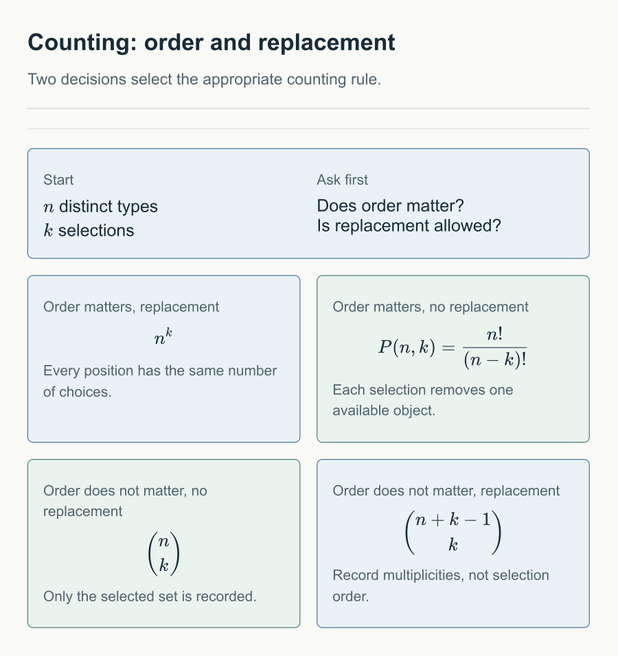
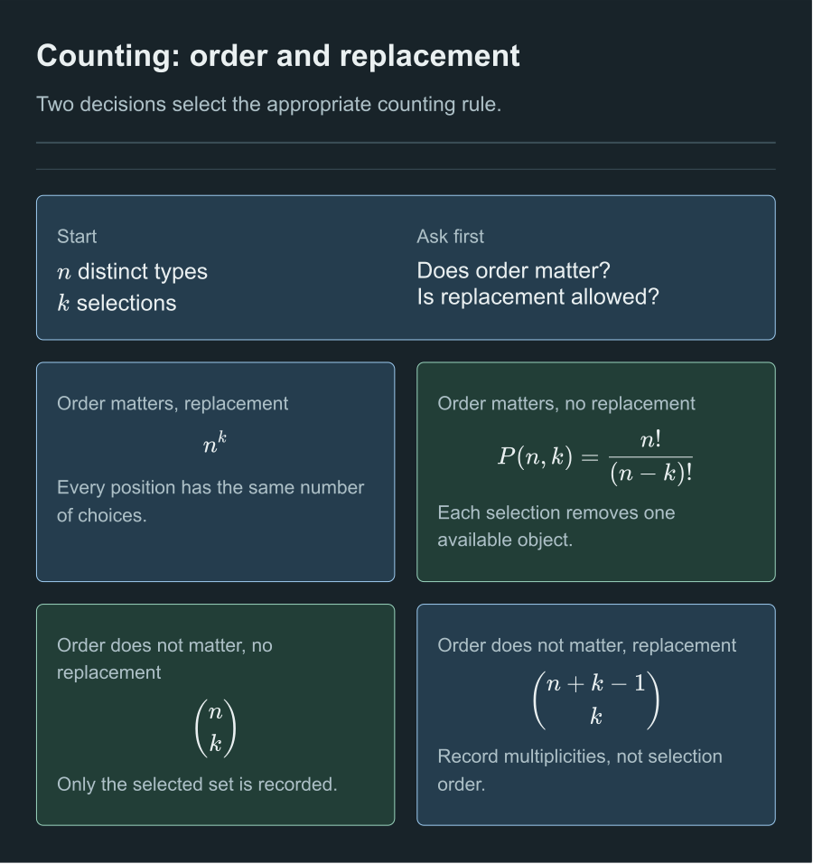
Choose a counting rule by asking whether order matters and whether repetition is allowed.

Permutation

We first introduce Permutation, which focuses on finding ways of arrangement for selection with order. Consider that the string $abc$. How many ways can we arrange them? But listing all the possibilities: $abc, acb, bac, bca, cab, ,cba$ we can tell that the answer is 6. For each of these results, we call it a Permutation for these letters.

Now we think about a more generalized case, where we have $n$ letters, where each letter is distinguishable, even though they are the same latter. Such as for $a_1$ and $a_2$ we have two permutations, $a_1a_2$ and $a_2a_1$.

We can actually apply this by product rule. Since for the first letter, we are choosing it from $n$ letters, giving $n$ choices, and the second one gives $n-1$ choices, so and and so forth, until we put the last remaining letter into the string. We have

$$n(n-1)(n-1)\dots 3\dots 2 \dots 1$$

which is also called $n$ factorial or full permutation.

Definition

Suppose now that we have $n$ objects. We have that there are

$$n\cdot (n-1)\dots \cdot2 \cdot 1 = n!$$

possible permutations.

Notation

The factorial of a non-negative integer $n$, denoted by $n!$, is the product of all positive integers less than or equal to $n$. It is defined as:

$$n! = n \times (n-1) \times (n-2) \times \cdots \times 2 \times 1$$

The factorial function grows very rapidly with the increase of $n$. It is used prominently in permutations and combinations, as well as in the calculation of probabilities and various mathematical series.

Additionally, by convention, the factorial of zero is defined as $0! = 1$. There will be an exercise on this.

We can combine the counting method for permutation with basic counting principals. Here is an example.

Example

A class in probability theory consists of 6 men and 4 women. An examination is given, and the students are ranked according to their performance. Assume that no two students obtain the same score. How many ways of ranking are possible? If the ranking are separated among boys and girls, how many ways of ranking are there?

Solution

First, we need to tell which kind of arrangement is involved. Obviously, ranking is ordered. So for the first case, we have $(6+4)! = 3628800$ cases. In the second case however, boys and girls are ranked separately. So we either rank girls first or rank boys first. We have $6!4! = 720\times 64 =17280$.

Remark

This example also shows that $\forall a,b\in \mathbb{Z}^+, (a+b)! \geq a!b!$.

Let's try out a different example.

Example

How many different letter arrangements can be formed from the letters PEPPER?

Solution

We first note that there are $6!$ permutations of the letters $P_1E_1P_2P_3E_2R$ when the 3P's and the 2E's are distinguished from one another. However, consider any one of these permutations, for instance, $P_1P_2E_1P_3E_2R$. If we now permute the P's among themselves and the E's among themselves, then the resultant arrangement would still be of the form PPEPER. That is, all 3! 2! permutations.

$$\begin{array}{ll}P_{1} P_{2} E_{1} P_{3} E_{2} R & P_{1} P_{2} E_{2} P_{3} E_{1} R \\P_{1} P_{3} E_{1} P_{2} E_{2} R & P_{1} P_{3} E_{2} P_{2} E_{1} R \\P_{2} P_{1} E_{1} P_{3} E_{2} R & P_{2} P_{1} E_{2} P_{3} E_{1} R \\P_{2} P_{3} E_{1} P_{1} E_{2} R & P_{2} P_{3} E_{2} P_{1} E_{1} R \\P_{3} P_{1} E_{1} P_{2} E_{2} R & P_{3} P_{1} E_{2} P_{2} E_{1} R \\P_{3} P_{2} E_{1} P_{1} E_{2} R & P_{3} P_{2} E_{2} P_{1} E_{1} R\end{array}$$

Since we know, the full permutation case where all letters are distinguished is interpreted by $6!$ which is a full permutation. Now what we will do is excluding the cases where confusion could be caused because of repeated letters using division Principal. Therefore the answer is $\frac{6!}{3!2!} = 60$, which means excluding all the cases with the same answer attributed to the repetition.

In this example, we combined Permutation counting with division rule. We call this kind of problems "Permutations with Repetition".

Definition

For the permutation problem with $n$ items, among which $n_1$, $n_2$, until $n_k$ are number of repetition within each item. The total number of permutation when not distinguishing repetition is

$$\frac{n!}{n_1! \cdot n_2! \cdot \ldots \cdot n_k!}.$$

Now we consider another example to introduce the specific permutation of a certain amount of element from a complete entity.

Example

Suppose we have 1, 2, 3, 4, four digits to generate any possible three-digit numbers, how many such numbers could be created (we will not remove any number after selection)?

Solution

Since all numbers can be used multiple times, we have 3 choices among 4 numbers, giving us $4\times 4 \times 4 = 64$ choices by product rule.

Now we change the scenario by removing the chosen number after each selection.

Example

Suppose we have 1, 2, 3, 4, four digits to generate any possible three-digit numbers, how many such numbers could be created (we will remove any number after selection)?

Solution

We first focus on choosing the number. Since now the number will not be replaced, we have $4\times 3 \times 2 = 24$ ways to choose the number, where each number has different sequence for the digits.

We see that the pattern in the second example is completely different from the first example by just changing one condition. This kind of irreplaceable permutation are categorized to $r$-Permutation.

Theorem

If $n$ is a positive integer and $r$ is an integer with $1\leq r\leq n$, then there are

$$P(n,r)=n(n-1)(n-2)\cdots(n-r+1)$$

$r$-permutations of a set with $n$ distinct elements. Note that another common notation for this is $^n P_r$.

Proof

Fill the ordered positions in sequence. After $j$ choices there are exactly $n-j$ unused elements, independent of which distinct prefix was chosen. Multiplying the counts for $j=0,\ldots,r-1$ gives the product. Cancelling the factors $1,\ldots,n-r$ from $n!$ gives the factorial quotient. For $r=0$ there is exactly one empty ordering, so the quotient still gives one.

But this open form is quite lengthy, can we write it in a closed form? Of course yes, because may already realize that the form of the expression is pretty similar to factorial. But the domain of the factorial function is $\N_0$(natural number greater or equal to 0), while $r\geq 1$ as mentioned in the theorem. By the definition of permutation, we know that $P(n,0)$ must evaluate to 1, for a similar reason to $0!=1$. By the division rule, we can get that $\frac{n!}{n!}=1$, which means we are not choosing anything from the entity. Now, if we introduce the variable $r\in[0,n]$ to the last expression, we get the closed form:

$$P(n,r) = \frac{n!}{(n-r)!}$$

.

Corollary

If $n$ and $r$ are integers with $0\leq r\leq n$, then $P(n,r)=\frac{n!}{(n-r)!}.$

The explanation above are more about reasoning, while this corollary can also be obtained by algebra analysis to $P(n,r)=n(n-1)(n-2)\cdots(n-r+1)$, since this can be taken as the quotient of some $n$ factorial divided by $n-r$ factorial.

This is exactly what we have been using in example numberselect.

Combination

Now we consider some other scenario of counting.

Example

how many possible combinations could be obtained by selecting 3 letters out of $a,b,c,d,e$ (non-replaceable), where the combination is not ordered, meaning that $ab\equiv ba$, both together count for 1 single case.

Solution

We know that we have 5 choices for the first letter and 4 choices for the second letter, 3 for the last one. so we have $5\times 4\times 3 = 60$. However, this includes some equivalent combinations, which we need to rule out.

We know that each result is a string of length 3, so we know that every $3!=6$ orderings of a selected triple form one equivalence class, which will be only counted once. To exclude them, we need to divide all result of selections with the full permutation of any possible string length 3, which is $3!$. So we have $\frac{5\times 4 \times 3}{3\times 2 \times 1} = 10$ cases.

This result is quite obvious, however, if you examine further, $5\times 4 \times 3 = P(5,3)$. So we can write it as $\frac{P(5,3)}{3!}$. We can use the same letter $n,r$ to denote this relation as

$$\frac{P(n,r)}{r!} = \frac{n!}{(n-r)!r!}.$$

We call this $r$-combination of $n$.

Theorem

The number of $r$-combinations of a group of object with $n$ distinct elements is denoted by $C(n,r)$ or $\binom{n}{r}$, and is called a binomial coefficient. We define $\binom{n}{r}$,for $r\leq n$, by

$$\binom{n}{r} = \frac{n!}{(n-r)!r!}$$

and say that $\binom{n}{r}$ (read as "$n$ choose $r$") represents the number of possible combinations of $n$ objects taken $r$ at a time.

Proof

Assume integers $0\le r\le n$. Every unordered $r$-subset produces exactly $r!$ distinct ordered selections. The fibers of the forget-order map therefore all have size $r!$, so the division rule gives $\binom nr=P(n,r)/r!$. This also covers $r=0$ using the empty selection.

Here is an example for your better understanding of this.

Example

From a group of 5 women and 7 men, how many different committees consisting of 2 women and 3 men can be formed? What if 2 of the men are feuding and refuse to serve on the committee together?

Solution

As there are $\binom{5}{2}$ possible groups of 2 women, and $\binom{7}{3}$ possible groups of 3 men, it follows from the basic principle that there are

$$\binom{5}{2} \times \binom{7}{3} = \frac{5 \cdot 4}{2 \cdot 1} \times \frac{7 \cdot 6 \cdot 5}{3 \cdot 2 \cdot 1} = 350$$

possible committees consisting of 2 women and 3 men.

Now suppose that 2 of the men refuse to serve together. There are $\binom{7}{3}=35$ groups in total, and exactly $\binom22\binom51=5$ contain both feuding men, it follows that there are $35 - \binom{2}{2} \times \binom{5}{1} = 30$ groups that do not contain both of the feuding men. Because there are still $\binom{5}{2} = 10$ ways to choose the 2 women, there are $30 \times 10 = 300$ possible committees in this case.

Do keep in mind that even with combination and permutation methods, the basic principles of counting are still essential for problem-solving.

Here's another important fact about binomial number.

Corollary

Let $n$ and $r$ be nonnegative integers with $r \leq n$. Then $C(n, r) = C(n, n - r)$.

Proof

From Theorem rcombi it follows that

$$C(n, r) = \frac{n!}{r!(n - r)!}$$

and

$$C(n, n - r) = \frac{n!}{(n - r)![n - (n - r)]!} = \frac{n!}{(n - r)!r!}.$$

Hence, $C(n, r) = C(n, n - r)$.

We also provide another combinatorial proof.

Proof

By definition, the number of subsets of S with $r$ elements equals $C(n,r)$. But each subset A of S is also determined by specifying which elements are not in $A$, and so are in $A$. Because the complement of a subset of $S$ with $r$ elements has $n-r$ elements, there are also $C(n,n-r)$ subsets of S with $r$ elements. It follows that $C(n,r)=C(n,n-r).$

Another interesting result is about decomposition of combination number.

Example

Suppose you are sent to buy 6 bananas. The store has 20 bananas altogether: 19 good ones and 1 bad one. Any selection of 6 either avoids the bad one or includes it. So the total number of selections equals the number containing only good bananas plus the number that contain the bad one and 5 good ones. That is,

$$\begin{aligned} \binom{20}{6}& =\binom{19}6+\binom{19}5=\frac{19!}{6!\times13!}+\frac{19!}{5!\times14!} \\ &=\frac{19\times18\times17\times16\times15\times14}{6\times5\times4\times3\times2\times1}+\frac{19\times18\times17\times16\times15}{5\times4\times3\times2\times1} \\ &=19\times17\times2\times3\times14+19\times18\times17\times2 \\ &=27 132+11 628=38 760. \end{aligned}$$

This bring us to the following conclusion.

Corollary

This result applies in general, if $0<k<n$, then

$$\binom{n}{k} = \binom{n-1}{k-1} + \binom{n-1}{k}$$

Proof

$$\begin{aligned} &\begin{pmatrix}n-1\\k\end{pmatrix}+\begin{pmatrix}n-1\\k-1\end{pmatrix}=\frac{(n-1)!}{k!\times[(n-1)-k]!}+\frac{(n-1)!}{(k-1)!\times[(n-1)-(k-1)]!} \\ &=\frac{(n-1)!}{k!\times[n-k-1]!}+\frac{(n-1)!}{(k-1)!\times[n-k]!}\\ &=\frac{(n-1)!}{k!\times(n-k-1)!}\times\frac{(n-k)}{(n-k)}+\frac{k}{k}\times\frac{(n-1)!}{(k-1)!\times(n-k)!}\quad\\ &=\frac{[(n-k)+k]\times(n-1)!}{k!:\times:(n-k)!}=\frac{n\times(n-1)!}{k!\times(n-k)!}=\frac{n!}{k!:\times:(n-k)!}=\left(\begin{aligned}n\\k\end{aligned}\right). \end{aligned}$$

You may have realized that this is a recursive relation. We will discuss more on this topic later.

Remark

This identity is called Pascal's Identity. You may find an interesting combinatorial proof in the link.

Further Interpretation of Counting with Set Theory

Now let's wrap up what we have covered in this section. We have gone through combination and permutations, and have seen many examples. However, we haven't reached the nature of these counting method. Fundamentally, all counting problems are set problems. Recall how the four principals of accounting are defined in the last section. Without conclusions and concepts in naive set theory, none of them will exist.

We have also seen the intricate relation between fundamental counting principals and permutation, as well as combination. Actually, set theory is one of the cornerstone of counting methods. For every problem we have solved so far, we are actually manipulating a set or multiple sets, and their members. This is because set or class is the abstraction of any existent objects that share some common property.

The way we distinguish different counting problems, or method we are going to use is basically by finding two properties of the problem.

• Whether it is a permutation or combination problem?

• Can each object be selected repetitively?

Now let's recap the four cases of counting and relate them to higher abstraction in sets.

$k$-Sequences on an $n$-Set

Definition

When the codomain of a sequence S is the set $C$, we say that S is a sequence on C If both $k$ and $n$ are positive integers, then a k-sequence on an an-set is a function S from $\{1..k\}$ into some set $X=\{x_1,x_2,\ldots,x_n\}$ with exactly $n$ elements, and we may write S as

$$S=(s_1,s_2,s_3,\ldots,s_k) \text{ where each } s_j\in X.$$

For $r$-permutation that allow repetition, we can take it as the number of $k$-Sequences on an $n$-Set. This means that we are choosing $k$ members from set $n$, and rearrange them to any possible sequence. Since we know that in a sequence, the same object that appears multiple times are distinguishable. So the total number of outcomes is $n^k$.

For example, there are $4^3$ 3-sequence on $\{1,2,3,4\}$.

For $r$-permutation that does not allow repetition, meaning that each element can only be chosen once. In this case we are trying to get a sequence of size $r$ where each member is unique and is from $C$. This can be perfectly fitted into the definition of $P(n,r)$. This is equivalent to "truncate" the full permutation ($(n-k)\times \dots \times 1$), so we have

$$n\times(n-1)\times \dots \times(n-k+1).$$

For example, The number of 4-permutations on a 6-set is

$$6\times 5 \times 4 \times 3=360.$$

We can actually also write the number of 6-permutations on 4-set, which is

$$4 \times 3\times 2\times 1 \times 0 \times (-1)=0.$$

Obviously it does not exist.

We have learned that the number of subset of a $n$-set is $2^n$. This is actually a corollary fundamental counting Principal. Because for any set with $n$ member (we call it $S$), we can define a characteristic sequence $X$(we discussed in set theory, chapter2), and the cardinality of the characteristic sequence must equal to $n$. Now considering the subsets. Each possible characteristic sequence map to a unique subset of the original set, and each position of $X$ can only be either 0 or 1, so $S$ have $2^n$ characteristic sequence, i.e., $S$ has $2^n$ subsets.

Number of $k$-Subsets of an $n$-Set

Now we consider number of $k$-subsets of an $n$-set. Since a set has no sequence and is not repetitive element, so we know that the number of result for non-repetitive $k$-Subsets of an $n$-Set is exactly $\binom{n}{r}$.

But how can we understand combination with repetition, also known as Multiset combination? Multiset combinations refer to combinations where repetition of elements is allowed. Unlike sets, where each element is unique, a multiset can contain multiple occurrences of the same element. Mathematically, we denote the number of $k$-combinations from a set with $n$ elements with repetition allowed as $\binom{n + k - 1}{k}$.

Definition

Given a set $X = \{x_1, x_2, \ldots, x_n\}$, a $k$-combination with repetition allowed from $X$ is a selection of $k$ elements from X where each element can appear multiple times. The total number of such combinations is given by:

$$\binom{n + k - 1}{k} = \frac{(n + k - 1)!}{k!(n - 1)!}$$

Proof

We model the problem of selecting $k$ elements from the multiset $X$ using the stars and bars method. In this method, we represent each selection by a star (*) and use bars (|) to separate the different types of elements in the multiset.

For $k$ selections and $n$ types of elements, we need $k$ stars and $n-1$ bars. The bars are used to partition the $k$ stars into $n$ distinct groups, where each group corresponds to one type of element from the multiset $X$.

The total number of symbols (stars and bars together) is $n + k - 1$. To find the number of ways to arrange these symbols, we need to choose $k$ positions for the stars out of the $n + k - 1$ available positions, leaving the remaining positions for the bars.

This is equivalent to choosing $k$ elements from a set of $n + k - 1$ elements, which is given by the binomial coefficient:

$$\binom{n+k-1}{k} = \frac{(n+k-1)!}{k!(n-1)!}$$

Thus, the number of $k$-subsets of an $n$-multiset, where repetition is allowed, is precisely the number of ways to arrange $k$ stars and $n-1$ bars, confirming the formula.

Here are some examples.

Example

Consider a set of fruits $F = \{ \text{apple}, \text{banana}, \text{cherry} \}$. If we want to select 2 fruits with repetition allowed, the possible combinations are:

• Two apples.

• One apple and one banana.

• One apple and one cherry.

• Two bananas.

• One banana and one cherry.

• Two cherries.

The number of combinations with repetition is $\binom{3 + 2 - 1}{2} = \binom{4}{2} = 6$.

Example

For choosing 3 balls from a set of balls with colors red (R), blue (B), and green (G), we have the following multiset combinations:

• RRR, RRB, RRG, RBB, RBG, RGG

• BBB, BBG, BGG, GGG

• RRR, BBB, GGG (repetitions of the same color)

By the formula, the number of combinations with repetition is $\binom{3 + 3 - 1}{3} = \binom{5}{3} = 10$.

Here is a brief wrap up for distinguishing these problems.

• $k$-subset of an $n$-set: In this scenario, the set consists of $n$ distinct elements, and we want to choose $k$ of them. No element can be chosen more than once because sets do not allow for repetition. The order of selection does not matter, and the total number of $k$-subsets is given by the binomial coefficient $\binom{n}{k}$.

• $k$-subset of an $n$-multiset: In contrast, a multiset can have repeated elements, so when we choose $k$ elements from an $n$-multiset, we are allowed to select the same element multiple times. This greatly increases the number of possible combinations since each of the $k$ slots can be filled with any of the $n$ elements, with repetitions. The total number of such combinations is given by $\binom{n+k-1}{k}$, which accounts for the possibility of repetition.

Example

Consider a set $S$ of 5 distinct books. If we want to select 3 books to place on a shelf, we use combinations without repetition. The total number of ways to do this is given by:

$$\binom{5}{3} = \frac{5!}{3!(5-3)!} = 10.$$

Now, consider a multiset $M$ of 5 types of fruits with an unlimited quantity of each type. If we want to select a basket of 3 fruits, where we can select the same type more than once, we use combinations with repetition. The total number of ways to do this is given by:

$$\binom{5+3-1}{3} = \binom{7}{3} = \frac{7!}{3!(7-3)!} = 35.$$

When counting selections from a set, we use combinations without repetition because each element can be chosen only once. In contrast, when counting selections from a multiset, we use combinations with repetition since each element can appear multiple times in a selection.

Binomial Theorem

In previous section, we introduced corollary refpascal's identity. This conclusion is the foundation of binomial theorem, which is why we call $\binom{n}{r}$ binomial coefficient. We have learned in the middle school the basic algebra knowledge that $(a\pm b)^2 = a^2 \pm 2ab + b^2$ Though we can prove it by using basic algebra, but it does not really matter here. This conclusion is only a subconclusion of its further generelization, and we call it Binomial Theorem.

Theorem

All binomials with $x\in \mathbb{R}\space \text{and}\space y\in \mathbb{R}$ with $n \in \mathbb{Z}$ follow:

$$(x+y)^{n}=\sum_{k=0}^{n}\left(\begin{aligned}n \\k\end{aligned}\right) x^{k} y^{n-k}$$

This theorem could be proven easily by induction with corollary pascal's identity as lemma.

Proof

For the base case of $n = 1$, $(x+y)^1 = \binom{1}{0} x^0y^1 + \binom{1}{1}x^1y^0 = x+y$ With this suppose when $n = n- 1$, by theorem BT:

$$(x+y)^{n-1} = \sum_{k=0}^{n-1}\left(\begin{aligned}n-1 \\k\end{aligned}\right) x^{k} y^{n-1-k}$$

While

$$(x+y)^n = (x+y)(x+y)^{n-1} = (x+y)\sum_{k=0}^{n-1}\left(\begin{aligned}n-1 \\k\end{aligned}\right) x^{k} y^{n-1-k}$$$$= \sum_{k=0}^{n-1}\left(\begin{aligned}n-1 \\k\end{aligned}\right) x^{k+1} y^{n-1-k} + \sum_{k=0}^{n-1}\left(\begin{aligned}n-1 \\k\end{aligned}\right) x^{k} y^{n-k} \space \text{(Distribution Law)}$$

Let $i = k+1$ in the first sum and $i=k$ in the second sum:

$$\begin{aligned}(x+y)^{n} & =\sum_{i=1}^{n}\left(\begin{aligned}n-1 \\i-1\end{aligned}\right) x^{i} y^{n-i}+\sum_{i=0}^{n-1}\left(\begin{aligned}n-1 \\i\end{aligned}\right) x^{i} y^{n-i} \\& =x^{n}+\sum_{i=1}^{n-1}\left[\left(\begin{aligned}n-1 \\i-1\end{aligned}\right)+\left(\begin{aligned}n-1 \\i\end{aligned}\right)\right] x^{i} y^{n-i}+y^{n} \\& =x^{n}+\sum_{i=1}^{n-1}\left(\begin{aligned}n \\i\end{aligned}\right) x^{i} y^{n-i}+y^{n} \\& =\sum_{i=0}^{n}\left(\begin{aligned}n \\i\end{aligned}\right) x^{i} y^{n-i}\end{aligned}$$

Thus the theoremBT is proved.

But actually we can get a more concise and elegant combinatorial proof, you may check here.

Example

The binomial theorem states that for any positive integer $n$, the expansion of $(a+b)^n$ is given by:

$$(a + b)^n = \sum_{k=0}^{n} \binom{n}{k} a^{n-k} b^k$$

where $\binom{n}{k}$ are the binomial coefficients.

Remark

Why this looks different from the theorem? Think about it. Is it really a different expression? What if we are just interchange the notation for each number? Isn't it the same?

For $n=3$:

$$(a + b)^3 = \binom{3}{0}a^{3}b^{0} + \binom{3}{1}a^{2}b^{1} + \binom{3}{2}a^{1}b^{2} + \binom{3}{3}a^{0}b^{3}$$$$= a^{3} + 3a^{2}b + 3ab^{2} + b^{3}$$

For $n=4$:

$$(a + b)^4 = \binom{4}{0}a^{4}b^{0} + \binom{4}{1}a^{3}b^{1} + \binom{4}{2}a^{2}b^{2} + \binom{4}{3}a^{1}b^{3} + \binom{4}{4}a^{0}b^{4}$$$$= a^{4} + 4a^{3}b + 6a^{2}b^{2} + 4ab^{3} + b^{4}$$

For $n=5$:

$$(a + b)^5 = \binom{5}{0}a^{5}b^{0} + \binom{5}{1}a^{4}b^{1} + \binom{5}{2}a^{3}b^{2} + \binom{5}{3}a^{2}b^{3} + \binom{5}{4}a^{1}b^{4} + \binom{5}{5}a^{0}b^{5}$$$$= a^{5} + 5a^{4}b + 10a^{3}b^{2} + 10a^{2}b^{3} + 5ab^{4} + b^{5}$$

The coefficients in the expansion follow a pattern known as Pascal's triangle. Each coefficient is the sum of the two coefficients above it in the previous expansion. For instance, the coefficient of $a^{3}b^{2}$ in the expansion of $(a+b)^5$ is 10, which is the sum of the coefficients of $a^{4}b^{1}$ and $a^{3}b^{2}$ from the expansion of $(a+b)^4$, which are 4 and 6, respectively. You may see more here.

In the last section, we used combinatorial proof to explain why the number of subsets for a $n$-set is $2^n$. Now we can get one more way to explain it by Binomial Theorem.

Proof

Since there are $\binom{n}{k}$ subsets of size $k$, So by theorem BT

$$\sum_{k=0}^{n}\binom{n}{k}=(1+1)^n = 2^n.$$

Multinomial Theorem

The name of this chapter have told you that our discussion on the power of sum of numbers does not end here. Mathematicians seek to generalize every problem, so as computer scientists and programmers. Now suppose we want to find the pattern of result of some expression involving more than 3 numbers or variables $(a+b+c)^n$, how can we get the expansion?

Before we do that, let's considering such scenario.

Example

How many ways can you arrange the letters in the word "SUCCESS"? Since the word "SUCCESS" has 7 letters with 1 "S", 1 "U", 2 "C", and 3 "S", the number of arrangements is given by the multinomial coefficient:

$$\binom{7}{1,1,2,3} = \frac{7!}{1! \cdot 1! \cdot 2! \cdot 3!} = 420.$$

Example

Consider a set of $n$ distinct items to be divided into $r$ distinct groups of respective sizes $n_1, n_2, \ldots, n_r$, where $\sum_{i=1}^{r} n_i = n$. The number of ways to perform this division is given by the multinomial coefficient:

$$\binom{n}{n_1, n_2, \ldots, n_r} = \frac{n!}{n_1! \cdot n_2! \cdot \ldots \cdot n_r!}$$

This is derived from the principle of counting, starting with $\binom{n}{n_1}$ ways to choose the first group, then $\binom{n - n_1}{n_2}$ ways for the second, and so on, leading to the product of binomial coefficients which simplifies to the formula above due to the factorial terms canceling out. Each division corresponds to a unique permutation of the items into the groups, considering items within the same group as indistinguishable.

We have covered similar problems earlier as permutation without repetition. Here we introduce a new notation for this.

Notation

If $n_1 + n_2 + \dots + n_r = n$, we define $\binom{n}{n_1, n_2, \ldots, n_r}$ by

$$\binom{n}{n_1, n_2, \ldots, n_r} = \frac{n!}{n_1! \cdot n_2! \cdot \ldots \cdot n_r!}.$$

Thus, $\binom{n}{n_1, n_2, \ldots, n_r}$ represents the number of possible divisions of $n$ distinct objects into $r$ distinct groups of respective sizes $n_1, n_2, \ldots, n_r$.

We call this Multinomial Coefficient. This allows us to generalize Multinomial Theorem.

Definition

The multinomial theorem extends the binomial theorem to polynomials with any number of terms. For any positive integer $n$ and non-negative integers $n_1, n_2, \ldots, n_k$ such that $n_1 + n_2 + \cdots + n_k = n$, the theorem states that:

$$(a_1 + a_2 + \cdots + a_k)^n = \sum \binom{n}{n_1, n_2, \ldots, n_k} \cdot a_1^{n_1} \cdot a_2^{n_2} \cdots a_k^{n_k},$$

We only offer the combinatorial proof here, since the induction proof could be made easily by binomial theorem. That will be one of the exercises.

Proof

The multinomial coefficient $\binom{n}{n_1, n_2, \ldots, n_k}$ counts the number of ways to partition a set of $n$ distinct items into $k$ bins with $n_i$ items in the $i$-th bin. This corresponds to the number of distinct sequences that can be formed by permuting the $n$ items where there are $n_i$ of the $i$-th type.

When we expand $(x_1 + x_2 + \cdots + x_k)^n$ by distributing and multiplying out all terms, each term in the expansion corresponds to choosing one of the $x_i$'s from each of the $n$ factors. The coefficient of a given term $x_1^{n_1} x_2^{n_2} \cdots x_k^{n_k}$ in the expanded product corresponds to the number of sequences of these choices, which is precisely the multinomial coefficient.

Hence, the combinatorial interpretation of the multinomial coefficients directly provides a proof of the multinomial theorem.

The multinomial theorem is related to permutations with repetition. Permutations with repetition occur when we want to count the number of different sequences that can be formed with a set of $n$ elements where each element can appear multiple times. The number of such permutations is given by the multinomial coefficient. This is because each term in the expansion represents a unique way to permute the $n$ objects into $k$ distinct groups with $n_1, n_2, \ldots, n_k$ objects in each group, with the condition that some objects may be identical to one another.

Example

Expanding $(a + b + c)^4$ using the multinomial theorem gives:

$$(a + b + c)^4 = \binom{4}{4,0,0}a^4 + \binom{4}{3,1,0}a^3b + \binom{4}{3,0,1}a^3c + \binom{4}{2,2,0}a^2b^2 + \ldots + \binom{4}{0,0,4}c^4$$

which simplifies to: $a^4 + 4a^3b + 4a^3c + 6a^2b^2 + 6a^2bc + 6a^2c^2 + 4ab^3 + 12ab^2c + 12abc^2 + 4ac^3 + b^4 + 4b^3c + 6b^2c^2 + 4bc^3 + c^4.$

Catalan Numbers

Section Pending Migration / Draft Placeholder

This subsection on Catalan numbers ($C_n = \frac{1}{n+1}\binom{2n}{n}$), Dyck paths, and balanced parenthesis counting is an outline placeholder queued for full exposition.

String Number Counting

Section Pending Migration / Draft Placeholder

This subsection on string arrangements and word permutations is an outline placeholder queued for full exposition.

Exercises

Exercise

We mentioned that $0!=1$ is defined purposely. Why it cannot be 0? Justify or refute it in any way you can work out.

Solution

Here are some possible explanations.

• Since factorial $n$ represents the way of ordered arrangement for $n$ objects, for 0 objects, we only have one way of arranging.

• $n!=n(n-1)!$, so we need to make sure $1 = 1(0)!$ exists, and therefore we $0!=1$

Exercise

Define a function $f: \mathbb{N}_0 \rightarrow \mathbb{N}_0$ by the following recursive relation:

$$f(n) = \begin{cases} 1 & \text{if } n = 0, \\ n \cdot f(f(n-1)) & \text{if } n > 0. \end{cases}$$

1. Prove or disprove: The function $f(n)$ is always equal to $n!$.

2. If $f(n)$ does not always equal $n!$, find an explicit expression for $f(n)$ and provide examples that demonstrate how $f(n)$ deviates from $n!$.

Hint: Compare this function with the strictly defined factorial recursive function.

Exercise

Prove that If $n$ is a positive integer and $r$ is an integer with $1\leq r\leq n$, then there are

$$P(n,r)=n(n-1)(n-2)\cdots(n-r+1).$$

Proof

We will use the product rule to prove that this formula is correct. The first element of the permutation can be chosen in $n$ ways because there are $n$ elements in the set. There are $n-1$ ways to choose the second element of the permutation, because there are $n-1$ elements left in the set after using the element picked for the first position. Similarly, there are $n-2$ ways to choose the third element, and so on, until there are exactly $n-(r-1)=n-r+1$ ways to choose the $r$th element. Consequently, by the product rule, there are

$$n(n-1)(n-2)\cdots(n-r+1)$$

$r$-permutations of the set.

Exercise

How many letter arrangements can be made from the letters

1. Fluke?

2. Propose?

3. Mississippi?

4. Arrange?

Solution

We can find the number of different arrangements of the letters by considering the factorials of the total number of letters divided by the factorials of the number of repeated letters.

1. For the word Fluke, there are no repeating letters. So, the number of different arrangements is simply $5!$:

$$5! = 5 \times 4 \times 3 \times 2 \times 1 = 120.$$

2. For the word Propose, the letter 'P' is repeated twice and the rest are distinct. So, the number of arrangements is:

$$\frac{7!}{2!} = \frac{7 \times 6 \times 5 \times 4 \times 3 \times 2 \times 1}{2 \times 1} = 2520.$$

3. In the word Mississippi, we have 'S' repeated four times, 'I' repeated four times, and 'P' repeated twice. The total number of arrangements is:

$$\frac{11!}{4!4!2!} = \frac{11 \times 10 \times 9 \times 8 \times 7 \times 6 \times 5 \times 4 \times 3 \times 2 \times 1}{(4 \times 3 \times 2 \times 1)(4 \times 3 \times 2 \times 1)(2 \times 1)} = 34650.$$

4. For the word Arrange, the letter 'A' is repeated twice, and the letter 'R' is repeated twice. The number of different arrangements is:

$$\frac{7!}{2!2!} = \frac{7 \times 6 \times 5 \times 4 \times 3 \times 2 \times 1}{(2 \times 1)(2 \times 1)} = 1260.$$

In each of these cases, we use the formula for permutations of n items with repetition, $\frac{n!}{n_1! \times n_2! \times \ldots \times n_k!}$, where $n_i$ is the number of times the ith element is repeated.

Exercise

Answer the following questions.

1. How many ways can a president, treasurer, and secretary be chosen from a group of 10 people?

2. How many ways can a team of three people be chosen from a group of 10 people?

3. What's the essential difference between (a) and (b)? Which answer is larger? Could you have known this without doing any calculation?

4. How many ways can a bowl of three scoops of ice-cream be selected from 10 flavours? (Multiple scoops of the same flavour are allowed.)

5. How many ways can five different prizes be divided among Anastasia, Becky, and Cadel? (Not everyone has to get a prize.)

6. In how many different orders can six horses finish a race? (Assume there are no ties and they all do finish.)

Solution

For question (a), since the roles are distinct and order matters, we use permutations. The number of ways is given by $P(10, 3)$.

$$P(10, 3) = \frac{10!}{(10-3)!} = 10 \times 9 \times 8 = 720.$$

For question (b), as order does not matter, we use combinations. The number of ways is given by $\binom{10}{3}$.

$$\binom{10}{3} = \frac{10!}{3!7!} = \frac{10 \times 9 \times 8}{3 \times 2 \times 1} = 120.$$

For question (c), the essential difference lies in the consideration of order. (a) uses permutations and is thus larger. Without calculations, we could deduce this due to the nature of permutations yielding more outcomes than combinations when order is taken into account.

For question (d), concerning the selection of ice-cream scoops, we consider two cases:

Case 1: Order of scoops matters. Each of the three scoops can be one of 10 flavours, and the order in which the flavours are chosen matters. In this case, each scoop is distinct, and the number of ways to select the ice-cream is $10^3$.

$$10^3 = 1000.$$

Case 2: Order of scoops does not matter. We are interested in the combination of flavours regardless of the order. This is a problem of combinations with repetition. The number of ways to select the ice-cream is given by the formula for combinations with repetition:

$$\binom{n + k - 1}{k}$$

where $n$ is the number of options (flavours), and $k$ is the number of selections (scoops). Here, $n = 10$ and $k = 3$:

$$\binom{10 + 3 - 1}{3} = \binom{12}{3} = \frac{12!}{3!9!} = \frac{12 \times 11 \times 10}{3 \times 2 \times 1} = 220.$$

So there are 220 different combinations if we do not consider the order of scoops.

For question (e), each of the five prizes can be awarded to any one of the three people independently, resulting in $3^5$ ways.

$$3^5 = 243.$$

For question (f), every horse finishing in a unique position is a permutation of 6 items.

$$6! = 720.$$

Exercise

Prove Multinomial Theorem by induction with Binomial Theorem

Solution

the multinomial theorem states:

$$(x_1 + x_2 + \cdots + x_k)^n = \sum \binom{n}{n_1, n_2, \ldots, n_k} x_1^{n_1} x_2^{n_2} \cdots x_k^{n_k},$$

where the sum is taken over all sequences of non-negative integer indices $n_1, n_2, \ldots, n_k$ such that $n_1 + n_2 + \cdots + n_k = n$.

Proof

We will prove the multinomial theorem by induction on the number of terms $k$.

Base Case ($k=2$): For $k=2$, the theorem reduces to the binomial theorem, which is already known to be true. That is,

$$(x_1 + x_2)^n = \sum_{i=0}^{n} \binom{n}{i} x_1^{n-i} x_2^i.$$

Inductive Step: Assume the theorem holds for some $k \geq 2$. We must show it also holds for $k+1$. Consider the expression $(x_1 + x_2 + \cdots + x_k + x_{k+1})^n$. We can write this as:

$$\left((x_1 + x_2 + \cdots + x_k) + x_{k+1}\right)^n.$$

By the binomial theorem, this is equal to:

$$\sum_{i=0}^{n} \binom{n}{i} (x_1 + x_2 + \cdots + x_k)^{n-i} x_{k+1}^i.$$

By the induction hypothesis, each term $(x_1 + x_2 + \cdots + x_k)^{n-i}$ can be expanded as:

$$\sum \binom{n-i}{n_1, n_2, \ldots, n_k} x_1^{n_1} x_2^{n_2} \cdots x_k^{n_k},$$

where the sum is taken over all sequences of non-negative integer indices $n_1, n_2, \ldots, n_k$ such that $n_1 + n_2 + \cdots + n_k = n-i$.

Thus, the entire expression expands to:

$$\sum_{i=0}^{n} \binom{n}{i} \sum \binom{n-i}{n_1, n_2, \ldots, n_k} x_1^{n_1} x_2^{n_2} \cdots x_k^{n_k} x_{k+1}^i,$$

where the outer sum is taken over $i$ and the inner sum is taken over $n_1, n_2, \ldots, n_k$.

This is the multinomial expansion for $k+1$ terms. By the principle of mathematical induction, the theorem is proved.

Axioms of Probability

In previous sections, we have solved the problem that how many outcomes can a certain event have under given conditions. This section introduces the concept of the probability of an event and then show how probabilities can be computed in certain situations.

Sample Space and Events

We have discussed the example of rolling a die in previous sections. Intuitively we know that the probability of getting the number 3 is 1/6 because it's one case out of all six cases. In this example, the possible results of the event (rolling a die to get a number) can be written as a set $S = \{1,2,3,4,5,6\}$, and therefore, the possibility of getting a certain number from 1 to 6 is $\frac{1}{|S|} = \frac{1}{6}$.

In this example, we call the set of all possible outcomes Sample Space, and getting 3 from the dice is an event. An event could be subset of the sample space.

Definition

The sample space $S$ of an experiment or random trial is the set of all possible outcomes of that experiment. Each outcome in $S$ is mutually exclusive and collectively exhaustive.

Definition

An event is any subset of the sample space $S$ and represents a collection of possible outcomes of the experiment. An event can be as small as containing no outcomes (null event $\emptyset$) or as large as the entire sample space.

Example

Consider an experiment where one card is drawn from a standard deck of 52 cards.

The sample space $S$ consists of 52 elements, each representing a unique card from the deck.

Example events could include:

• Event $D$: Drawing a face card (Jack, Queen, or King).

• Event $E$: Drawing a card of hearts.

• Event $F$: Drawing an ace.

Example

Consider a simple experiment where a fair coin is flipped twice.

The sample space for this experiment, denoted as $S$, is:

$$S = \{HH, HT, TH, TT\}$$

Here, $H$ stands for heads and $T$ for tails, with each element representing an outcome sequence over the two flips.

Example events could include:

• Event $G$: Getting at least one head.

$$G = \{HH, HT, TH\}$$

• Event $H$: Getting a tail for second trial.

$$H = \{HT, TT\}$$

Now that we know both sample space and events are sets. Set opperations are applicable for them. We use last example for further illustration. Now suppose we want to get the event that among the two trial, we have at least one head and no tail for second trial. All we need to do is taking the intersection of $G$ and $H$.

$$G\cap H = \{HT\}$$

So we have only one case which is $HT$ for this. The same goes for the union.

Remark

Additionally, intsersection of two events are sometimes conventionally written without intersection notation $\cap$, instead we have $GH \equiv G\cap H$.

Here we introduce some new notations for set representation in probability theory. Note that they are using the same notation as in what we have discussed in class (section intofclass), do differenciate them.

For some scenario where we may find the huge number of events, we use similar notation as $\Sigma$ and $\Pi$ to express cpnsecutive set operation.

Notation

Given an infinite sequence of events $\{E_n\}_{n=1}^{\infty}$, the union of these events is denoted by $\bigcup_{n=1}^{\infty} E_n$ and is the event containing all outcomes that are in at least one of the events $E_n$. Formally, an outcome $\omega$ is in $\bigcup_{n=1}^{\infty} E_n$ if and only if there exists at least one $n$ such that $\omega \in E_n$.

Similarly, the intersection of these events is denoted by $\bigcap_{n=1}^{\infty} E_n$ and is the event containing only those outcomes that are in every $E_n$. An outcome $\omega$ is in $\bigcap_{n=1}^{\infty} E_n$ if and only if for all $n$, $\omega \in E_n$.

Also, we use $^c$ to show complement event. In last example, we have $H^c = S-H = \{HH,TH\}$.

Here is an example to let you have some further understanding of the notation.

Example

We have learned demorgan's law in Boolean algebra and set theory, but only in a base case, meaning it volves only two sets or Boolean variables. We can use $\bigcap, \bigcup$ to interprete it as:

$$\begin{aligned}&\left(\bigcup_{i=1}^nE_i\right)^c=\bigcap_{i=1}^nE_i^c\\&\left(\bigcap_{i=1}^nE_i\right)^c=\bigcup_{i=1}^nE_i^c.\end{aligned}$$

Remark

Do remember that for some set $S$, $S^c, S^\prime,\bar{S}$ are the same thing.

Probability Axioms

This section introduces axioms of probability theorey and some useful propositions. Before that, we need to define what is probability. In natural language you may say, probability is the chance that a certain thing happen, which is intollerable for mathematicians. Here are some common definitions.

Definition

The probability of an event is defined as the limit of its relative frequency in many trials. If an event $E$ occurs $n_E$ times in $n$ trials, the probability of $E$, $P(E)$, is given by:

$$P(E) = \lim_{n \to \infty} \frac{n_E}{n}$$

assuming the limit exists.

Definition

In the classical definition, applicable only to equally likely outcomes, the probability of an event $E$ is the ratio of the number of outcomes favorable to $E$ to the total number of possible outcomes in the sample space $S$. If $S$ is finite and each outcome is equally likely, then:

$$P(E) = \frac{|E|}{|S|}$$

where $|E|$ is the number of elements in $E$ and $|S|$ is the number of elements in $S$.

But don't need to delve into the definition too deep as it may involve something beyond this book. Either of these definitions are enough for solving basic probability problems.

Probability theory is a mathematical framework for quantifying uncertainty. It provides a set of formal principles, known as probability axioms, which underlie the entire structure of probability. These axioms were introduced by the Russian mathematician Andrey Kolmogorov in 1933, and they form the foundation upon which the modern theory of probability is built. The axioms are intended to be consistent and complete, and any mathematical system that satisfies these axioms is deemed a valid probability space. We discuss these axioms in detail below.

Axiom

For any event $E$ in the sample space $S$, the probability of $E$ is a non-negative number:

$$0\leq P(E) \leq 1.$$

Axiom

The probability of the entire sample space is 1:

$$P(S) = 1.$$

Axiom

For any sequence of disjoint events $\{E_i\}_{i=1}^n$ (events with no common outcomes), the probability of the union of these events is equal to the sum of their individual probabilities:

$$P\left(\bigcup_{i=1}^{\infty} E_i\right) = \sum_{i=1}^{\infty} P(E_i).$$

This is sometimes referred to as countable additivity.

With these axioms, we derive some other propositions for problem-solving. They are actually just some easy-to-find result from set theory.

Proposition

For any event $E$ in a probability space, the probability of the complement of $E$, denoted $E^c$, is given by:

$$P(E^c) = 1 - P(E).$$

This states that the likelihood of the event not occurring is the complement of the probability of the event occurring.

Proof

The sample space $S$ can be partitioned into two disjoint events, $E$ and its complement $E^c$. According to the axioms of probability, we have $P(S) = P(E) + P(E^c) = 1$. Therefore, rearranging for $P(E^c)$, we obtain $P(E^c) = 1 - P(E)$.

Proposition

If an event $E$ is a subset of event $F$, denoted $E \subseteq F$, then the probability of $E$ is less than or equal to the probability of $F$:

$$P(E) \leq P(F).$$

Proof

Given $E \subseteq F$, we can express $F$ as $F = E \cup (F \setminus E)$, where $F \setminus E$ is the set of all elements in $F$ that are not in $E$, effectively $E^c \cap F$. As $E$ and $F \setminus E$ are disjoint, from the axioms of probability, particularly countable additivity, we have:

$$P(F) = P(E) + P(F \setminus E)$$

Since probabilities are non-negative, $P(F \setminus E) \geq 0$, hence $P(E) \leq P(F)$.

Proposition

For any two events $E$ and $F$, the probability of their union is:

$$P(E \cup F) = P(E) + P(F) - P(E \cap F).$$

This formula accounts for the overlap between $E$ and $F$ to avoid double-counting.

Proof

The events $E$ and $F^c \cap F$ are disjoint, and their union is $E \cup F$. Applying the axiom of countable additivity, we have:

$$P(E \cup F) = P(E \cup (F^c \cap F)) = P(E) + P(F^c \cap F).$$

To find $P(F^c \cap F)$, note that it represents all outcomes in $F$ that are not in $E$, which is equivalent to $P(F) - P(E \cap F)$. Thus, we conclude:

$$P(E \cup F) = P(E) + P(F) - P(E \cap F).$$

We introduced the Principle of inclusion-exclusion of two sets in set theory (see theorem IE). Now we will prove it's generalized form so that we can use it for probability problems.

Theorem

For any collection of finite sets $A_1, A_2, \ldots, A_n$, the size of their union is given by: $\left|\bigcup_{i=1}^{n} A_i\right| = \sum_{\emptyset \neq I \subseteq [n]} (-1)^{|I|+1} \left|\bigcap_{i \in I} A_i\right|.$

Proof

Let $X$ denote a universal set that contains all the elements we are considering, and let $[n]$ represent the index set $\{1, 2, \ldots, n\}$. For any index set $I \subseteq [n]$, the expression $\bigcap_{i \in I} A_i$ denotes the intersection of those sets $A_i$ for which the index $i$ is in $I$.

For each set $A_i$ included in our universal set $X$, we define a characteristic function $f_i(x)$ as follows:

$$f_i(x) = \begin{cases} 1 & \text{if } x \in A_i, \\ 0 & \text{if } x \notin A_i. \end{cases}$$

We then consider the function $F(x)$ defined as the product of $1 - f_i(x)$ for $i$ from 1 to $n$:

$$F(x) = \prod_{i=1}^{n} (1 - f_i(x)).$$

This function $F(x)$ essentially acts as the characteristic function of the complement of the union of all sets $A_i$, taking the value 1 if and only if $x$ is not in any of the sets $A_i$.

Next, we express $F(x)$ by expanding the product into its individual terms:

$$F(x) = \prod_{i=1}^{n} (1 - f_i(x)) = \sum_{I \subseteq [n]} (-1)^{|I|} \prod_{i \in I} f_i(x).$$

Here, $\prod_{i \in I} f_i(x)$ is the product of the values of $f_i(x)$ for all $i$ in $I$, which is the characteristic function for the intersection $\bigcap_{i \in I} A_i$.

Taking the sum of $F(x)$ over all $x \in X$, we have:

$$\sum_{x \in X} F(x) = \sum_{I \subseteq [n]} (-1)^{|I|} \left|\bigcap_{i \in I} A_i\right|.$$

Comparing this with the direct computation of the sum of $F(x)$ as the size of the complement of the union of all $A_i$, we can equate the two expressions to obtain:

$$\left|X \setminus \bigcup_{i=1}^{n} A_i\right| = \left|X\right| - \left|\bigcup_{i=1}^{n} A_i\right| = \sum_{I \subseteq [n]} (-1)^{|I|} \left|\bigcap_{i \in I} A_i\right|.$$

By including the empty set in our summation, we consider it as $\left|X\right|$, the size of the universal set, and follow the same pattern of alternation as prescribed by the Principle of Inclusion-Exclusion. This completes the proof.

The same indicator identity gives the probability form.

Theorem

For any collection of events $A_1, A_2, \ldots, A_n$ in a probability space, the probability of the union of these events is given by: $P\left(\bigcup_{i=1}^{n} A_i\right) = \sum_{\emptyset \neq I \subseteq [n]} (-1)^{|I|+1} P\left(\bigcap_{i \in I} A_i\right).$

Proof

The indicator identity is pointwise:

$$\mathbf1_{\cup_i A_i} =1-\prod_i(1-\mathbf1_{A_i}) =\sum_{\emptyset\ne I\subseteq[n]}(-1)^{|I|+1}\mathbf1_{\cap_{i\in I}A_i}.$$

Taking expectations gives the probability formula. All sums are finite, so no interchange of an infinite series is involved. This proof applies even when individual outcomes have probability zero.

Below is how to understand it from combinatorial perspective.

Consider a noninductive argument for the Principle of Inclusion-Exclusion as applied to probability. Assume we have a probability space and events $A_1, A_2, \ldots, A_n$ within this space. If an outcome of the sample space does not belong to any of the event sets $A_i$, then it has no impact on the calculation of the probability of the union of these events since it is not an element of any union or intersection of these sets.

Now, suppose an outcome occurs in exactly $m$ of the events $A_i$, where $m > 0$. The probability associated with this outcome contributes once to the probability of the union $P(\bigcup_{i} A_i)$ since it must belong to at least one of the events $A_i$.

However, when we calculate the probability of the union using the Principle of Inclusion-Exclusion, this outcome's probability is counted multiple times: once for each event it belongs to, then subtracted for each intersection of two events it belongs to, added again for each intersection of three events, and so on. This alternation of addition and subtraction continues, matching the pattern of the binomial expansion of $(1 - 1)^m$, which is zero. More precisely, for $m > 0$, the outcome's probability is included $\binom{m}{1}$ times for single sets, subtracted $\binom{m}{2}$ times for intersections of pairs, added $\binom{m}{3}$ times for triple intersections, and so on, up to $(-1)^{m+1}\binom{m}{m}$ for the intersection of all $m$ events.

Mathematically, this summation can be expressed as follows:

$$1 = \binom{m}{0} = \binom{m}{1} - \binom{m}{2} + \binom{m}{3} - \ldots + (-1)^m\binom{m}{m}.$$

Given that $(1 - 1)^m = 0$, the binomial theorem tells us that:

$$0 = (1 - 1)^m = \sum_{i=0}^{m} \binom{m}{i}(-1)^i = \binom{m}{0} - \binom{m}{1} + \binom{m}{2} - \ldots + (-1)^m\binom{m}{m}.$$

The summation of the binomial coefficients weighted by alternating signs is thus zero, mirroring the way an outcome's probability is counted in the Inclusion-Exclusion formula. Consequently, each outcome's probability is correctly accounted for once in the total probability of the union of the events, validating the principle.

Exercises

Exercise

This problem involves axiom of probability and some propositions of probability theory. With these, you should prove Boole's Inequality.

Theorem

Let $E_1, E_2, \ldots, E_n$ be events from a finite sample space. Then,

$$P\left(\bigcup_{i=1}^n E_i\right) \leq \sum_{i=1}^n P(E_i).$$

This can be proven by both MI and with the help of axioms of probability.

Proof

Proof by MI. We prove Boole's Inequality by induction on the number $n$ of events.

Base case: When $n = 1$, the inequality clearly holds as:

$$P\left(\bigcup_{i=1}^1 E_i\right) = P(E_1) \leq P(E_1).$$

Inductive step: Assume the inequality holds for $n$ events, i.e.,

$$P\left(\bigcup_{i=1}^n E_i\right) \leq \sum_{i=1}^n P(E_i).$$

We need to prove it for $n+1$ events. Consider:

$$\bigcup_{i=1}^{n+1} E_i = \left(\bigcup_{i=1}^n E_i\right) \cup E_{n+1}.$$

Using the subadditivity of probability, we have:

$$P\left(\bigcup_{i=1}^{n+1} E_i\right) = P\left(\left(\bigcup_{i=1}^n E_i\right) \cup E_{n+1}\right) \leq P\left(\bigcup_{i=1}^n E_i\right) + P(E_{n+1}).$$

Applying the induction hypothesis:

$$P\left(\bigcup_{i=1}^n E_i\right) \leq \sum_{i=1}^n P(E_i),$$

it follows that:

$$P\left(\bigcup_{i=1}^{n+1} E_i\right) \leq \sum_{i=1}^n P(E_i) + P(E_{n+1}) = \sum_{i=1}^{n+1} P(E_i).$$

This completes the induction.

Therefore, by mathematical induction, Boole's Inequality holds for any finite number $n$ of events.

Proof

Proof by Axiom of Probability. The proof employs the principle of inclusion-exclusion and the non-negativity of probability.

The probability of the union of any two events $E_1$ and $E_2$ satisfies

$$P(E_1 \cup E_2) = P(E_1) + P(E_2) - P(E_1 \cap E_2),$$

which, given $P(E_1 \cap E_2) \geq 0$, implies that

$$P(E_1 \cup E_2) \leq P(E_1) + P(E_2).$$

Extending this to $n$ events, we have by the subadditivity axiom:

$$P\left(\bigcup_{i=1}^n E_i\right) = P\left(\bigcup_{i=1}^{n-1} E_i \cup E_n\right) \leq P\left(\bigcup_{i=1}^{n-1} E_i\right) + P(E_n).$$

Assuming inductively that the inequality holds for the union of $n-1$ events, i.e.,

$$P\left(\bigcup_{i=1}^{n-1} E_i\right) \leq \sum_{i=1}^{n-1} P(E_i),$$

we then obtain

$$P\left(\bigcup_{i=1}^n E_i\right) \leq \sum_{i=1}^{n-1} P(E_i) + P(E_n) = \sum_{i=1}^n P(E_i),$$

as required.

Or you can also consider theorem PrIE that we must have something less than or equal to $\sum_{i=1}^{n}P(E_i)$.

Remark

Boole's Inequality becomes an equality if and only if the events $E_1, E_2, \ldots, E_n$ are mutually disjoint. When the events are disjoint, the intersection of any two events is the empty set, implying $P(E_i \cap E_j) = 0$ for all $i \neq j$. In this case, the probability of the union of these events equals the sum of their individual probabilities, i.e.,

$$P\left(\bigcup_{i=1}^n E_i\right) = \sum_{i=1}^n P(E_i).$$

This scenario highlights the additive nature of probability in the absence of overlapping outcomes among events. Understanding this condition is crucial as it underscores the distinction between collective and independent probabilistic occurrences, often a key concept in studies involving probability theory and its applications.

Exercise

Consider a loaded six-sided die where rolling a 3 is twice as likely as rolling any other individual number. Find the probability of each outcome when the die is rolled.

Solution

Let $p(x)$ denote the probability of rolling a number $x$ on the die. According to the problem, rolling a 3 is twice as likely as rolling any other number, which can be mathematically represented as:

$$p(3) = 2p(x) \quad \text{for } x \neq 3.$$

Since the die is fair except for the loading, the probabilities for numbers other than 3 are equal, implying:

$$p(1) = p(2) = p(4) = p(5) = p(6).$$

The total probability for all outcomes must sum to 1, thus we have:

$$p(1) + p(2) + p(3) + p(4) + p(5) + p(6) = 1.$$

Substituting the condition $p(3) = 2p(1)$ into the equation, we obtain:

$$5p(1) + 2p(1) = 1 \implies 7p(1) = 1 \implies p(1) = \frac{1}{7}.$$

Hence, the probability for each outcome is:

$$p(1) = p(2) = p(4) = p(5) = p(6) = \frac{1}{7} \quad \text{and} \quad p(3) = \frac{2}{7}.$$

Exercise

Suppose that $E$ and $F$ are events such that $p(E) = 0.8$ and $p(F) = 0.6$. Show that $p(E \cup F) \geq 0.8$ and $p(E \cap F) \geq 0.4$.

Solution

To solve this exercise, we start by considering the union and intersection of the events $E$ and $F$.

Firstly, note that the probability of the union of two events $E$ and $F$ can be found using the formula for the union of two sets:

$$p(E \cup F) = p(E) + p(F) - p(E \cap F).$$

Given that $p(E) = 0.8$ and $p(F) = 0.6$, substituting these values into the formula gives:

$$p(E \cup F) = 0.8 + 0.6 - p(E \cap F).$$

Since the probability of any event is at most 1, we have:

$$0.8 + 0.6 - p(E \cap F) \leq 1,$$

which simplifies to:

$$p(E \cap F) \geq 0.4.$$

Therefore, the probability of the intersection of $E$ and $F$ is at least 0.4.

With $p(E \cap F) \geq 0.4$, substituting back into the union formula, we find:

$$p(E \cup F) = 0.8 + 0.6 - p(E \cap F) \geq 0.8 + 0.6 - 0.4 = 1.0.$$

However, since the probability cannot exceed 1, we consider the minimum possible value of $p(E \cup F)$, which aligns with the maximum probability of either event:

$$p(E \cup F) \geq \max(p(E), p(F)) = \max(0.8, 0.6) = 0.8.$$

Thus, we have shown both that $p(E \cup F) \geq 0.8$ and $p(E \cap F) \geq 0.4$.

Exercise

The conclusion on the probability of intersected events could be further generalized to Bonferroni's Inequality.

Theorem

Let $E$ and $F$ be events. Then, the probability of their intersection is bounded by:

$$p(E \cap F) \geq p(E) + p(F) - 1.$$

You may find the proof quite easy.

Proof

To prove Bonferroni's inequality, start by using the principle of inclusion-exclusion for the union of two events:

$$p(E \cup F) = p(E) + p(F) - p(E \cap F).$$

Since the probability of any event cannot exceed 1, we have:

$$p(E \cup F) \leq 1.$$

Substituting the expression for $p(E \cup F)$ into the inequality gives:

$$p(E) + p(F) - p(E \cap F) \leq 1.$$

Rearranging this inequality, we find:

$$p(E \cap F) \geq p(E) + p(F) - 1.$$

This derivation shows that the probability of the intersection of the events $E$ and $F$ is at least the sum of the probabilities of $E$ and $F$ minus 1, thereby establishing Bonferroni's inequality.

Exercise

Use induction to generalize Bonferroni's inequality to $n$ events.

Theorem

Let $E_1, E_2, \ldots, E_n$ be events in a probability space. Then, the probability of the intersection of these events is bounded below by the sum of the probabilities of each event minus the number of events minus one, i.e.,

$$P\left(\bigcap_{i=1}^n E_i\right) \geq \sum_{i=1}^n P(E_i) - (n - 1).$$

Also consider other ways to prove this, i.e., inclusion-exclusion.

We can do this by weak induction, which is more than enough.

Proof

Proof by Weak Induction. We proceed by mathematical induction on the number of events, $n$.

Base case: For $n = 2$, the inequality reduces to

$$P(E_1 \cap E_2) \geq P(E_1) + P(E_2) - 1,$$

which is just the simple Bonferroni's inequality and is true by the principles of probability.

Inductive step: Assume that the inequality holds for $n = k$, i.e.,

$$P\left(\bigcap_{i=1}^k E_i\right) \geq \sum_{i=1}^k P(E_i) - (k - 1).$$

We need to show that the inequality holds for $n = k+1$. Consider,

$$P\left(\bigcap_{i=1}^{k+1} E_i\right) = P\left(\left(\bigcap_{i=1}^k E_i\right) \cap E_{k+1}\right).$$

By the probability of intersections,

$$P\left(\left(\bigcap_{i=1}^k E_i\right) \cap E_{k+1}\right) = P\left(\bigcap_{i=1}^k E_i\right) - P\left(\bigcap_{i=1}^k E_i \cap E_{k+1}^c\right).$$

Using the inductive hypothesis and subtracting the probability of the complement,

$$P\left(\bigcap_{i=1}^k E_i\right) \geq \sum_{i=1}^k P(E_i) - (k - 1),$$$$P\left(\bigcap_{i=1}^k E_i \cap E_{k+1}^c\right) \leq P\left(E_{k+1}^c\right) = 1 - P(E_{k+1}),$$$$P\left(\bigcap_{i=1}^{k+1} E_i\right) \geq \sum_{i=1}^k P(E_i) - (k - 1) + P(E_{k+1}) - 1.$$

Simplifying this,

$$P\left(\bigcap_{i=1}^{k+1} E_i\right) \geq \sum_{i=1}^{k+1} P(E_i) - k,$$

which completes the inductive step.

Therefore, by mathematical induction, the Generalized Bonferroni's Inequality holds for any $n \geq 2$.

However, we can actually start with $n=1$ as our base case and use strong induction, making our life much easier.

Proof

Proof by Strong Induction. We prove this by strong induction on $n$.

Base case ($n=1$): The inequality trivially holds because

$$P(E_1) \geq P(E_1) - 0.$$

Inductive step: Assume the inequality holds for $n = k$, i.e.,

$$P\left(\bigcap_{i=1}^k E_i\right) \geq \sum_{i=1}^k P(E_i) - (k - 1).$$

We need to prove that the statement is true for $n = k+1$. Consider the intersection of $k+1$ events as two groups:

$$P\left(\bigcap_{i=1}^{k+1} E_i\right) = P\left(\left(\bigcap_{i=1}^k E_i\right) \cap E_{k+1}\right).$$

Applying the probability of intersections, we have:

$$P\left(\left(\bigcap_{i=1}^k E_i\right) \cap E_{k+1}\right) \geq P\left(\bigcap_{i=1}^k E_i\right) + P(E_{k+1}) - 1,$$

Using the inductive hypothesis for the first $k$ events:

$$P\left(\bigcap_{i=1}^k E_i\right) \geq \sum_{i=1}^k P(E_i) - (k - 1),$$

Combine these results:

$$P\left(\bigcap_{i=1}^{k+1} E_i\right) \geq \left(\sum_{i=1}^k P(E_i) - (k - 1)\right) + P(E_{k+1}) - 1,$$

Simplify the right-hand side:

$$P\left(\bigcap_{i=1}^{k+1} E_i\right) \geq \sum_{i=1}^{k+1} P(E_i) - k.$$

This completes the inductive step. Thus, by strong induction, the Generalized Bonferroni's Inequality holds for any $n \geq 1$.

Remark

This reminds us that in mathematical proofs, both weak and strong induction methods are commonly used, each having its own strengths and suitable applications.

Weak Induction: This method, also known as ordinary mathematical induction, assumes the truth of a statement for $n=k$ to prove it for $n=k+1$. It is straightforward and effective, particularly when each case depends only on its immediate predecessor. This simplicity makes weak induction especially approachable for many basic proofs.

Strong Induction: Strong induction assumes that the statement is true for all integers less than or equal to $k$, and uses this to prove the statement for $n=k+1$. This method is advantageous when the problem requires information from all previous cases, as it provides a more robust foundation for the proof, particularly in complex sequences or recursive relationships.

The choice between these induction techniques depends on the problem structure and which method more clearly communicates the proof's logic. While strong induction offers a comprehensive approach suitable for complex or highly interdependent scenarios, weak induction's simplicity is beneficial for more straightforward cases.

We also have a more interesting way to do that, simply by using principle of inclusion-exclusion.

Proof

Proof by Inclusion-Exclusion. The proof uses the principle of inclusion-exclusion and the non-negativity of probabilities. We start by considering the inclusion-exclusion formula for the probability of the union of $n$ events, which is:

$$P\left(\bigcup_{i=1}^n E_i\right) = \sum_{k=1}^n (-1)^{k+1} \left(\sum_{1 \leq i_1 < \cdots < i_k \leq n} P(E_{i_1} \cap \cdots \cap E_{i_k})\right).$$

However, we need the probability of the intersection, $P\left(\bigcap_{i=1}^n E_i\right)$, not the union. We consider the complementary probability:

$$P\left(\bigcap_{i=1}^n E_i\right) = 1 - P\left(\bigcup_{i=1}^n E_i^c\right).$$

Using the inclusion-exclusion principle on $E_i^c$ (the complements), we get:

$$P\left(\bigcup_{i=1}^n E_i^c\right) \leq \sum_{i=1}^n P(E_i^c),$$

where $P(E_i^c) = 1 - P(E_i)$.

Substituting back, we find:

$$P\left(\bigcap_{i=1}^n E_i\right) = 1 - P\left(\bigcup_{i=1}^n E_i^c\right) \geq 1 - \sum_{i=1}^n (1 - P(E_i)).$$

Simplifying further:

$$P\left(\bigcap_{i=1}^n E_i\right) \geq 1 - n + \sum_{i=1}^n P(E_i) = \sum_{i=1}^n P(E_i) - (n - 1).$$

This concludes the proof.

Exercise

Show that if $E_1, E_2, \ldots$ is an infinite sequence of pairwise disjoint events in a sample space $S$, then

$$p\left(\bigcup_{i=1}^\infty E_i\right) = \sum_{i=1}^\infty p(E_i),$$

by taking limits.

Solution

To prove this, we begin by noting that for any finite $n$, the probability of the union of the first $n$ events in the sequence, by axiom additivity, is

$$p\left(\bigcup_{i=1}^n E_i\right) = \sum_{i=1}^n p(E_i).$$

Since $E_1, E_2, \ldots$ are pairwise disjoint, this relationship holds due to the finite additivity of probability measures.

We now consider the limit as $n$ approaches infinity. By the definition of an infinite series and the continuity of probability measures from below (which is a standard result in measure theory, assuming non-decreasing sequences of sets),

$$p\left(\bigcup_{i=1}^\infty E_i\right) = \lim_{n \to \infty} p\left(\bigcup_{i=1}^n E_i\right).$$

Applying the limit to both sides of the equation established for the finite case,

$$\lim_{n \to \infty} p\left(\bigcup_{i=1}^n E_i\right) = \lim_{n \to \infty} \sum_{i=1}^n p(E_i) = \sum_{i=1}^\infty p(E_i),$$

where the last equality is justified by the definition of an infinite series sum.

Therefore, the probability of the union of an infinite sequence of pairwise disjoint events is equal to the sum of their individual probabilities.

Exercise

Two dice are thrown. Let $E$ be the event that the sum of the dice is odd, let $F$ be the event that at least one of the dice lands on 1, and let $G$ be the event that the sum is 5. Describe the events $EF$, $E \cup F$, $FG$, $EF^c$, and $EFG$.

Solution

Event Descriptions:

• $EF$ (Intersection of $E$ and $F$): This event represents both dice summing to an odd number and at least one die landing on 1. Possible outcomes include

$$\{(1, 2), (1, 4), (1, 6), (2, 1), (4, 1), (6, 1)\}$$

.

• $E \cup F$ (Union of $E$ and $F$): This event occurs if the sum is odd or if at least one of the dice lands on 1. Since $F$ includes any outcome with a 1, and $E$ includes all combinations leading to an odd sum, combining these covers a large set of possibilities, particularly those where at least one die results affect either condition.

• $FG$ (Intersection of $F$ and $G$): This event includes outcomes where at least one die is 1 and the sum is 5. Outcomes are $\{(1, 4), (4, 1)\}$ since these are the only ways to achieve a sum of 5 with at least one die showing 1.

• $EF^c$ (Intersection of $E$ and the complement of $F$): This event occurs when the sum is odd and neither die lands on 1. This excludes any odd sums involving a 1, narrowing the possibilities.

• $EFG$ (Intersection of $E$, $F$, and $G$): Since $G$ specifically requires the sum to be 5, and $F$ requires at least one die to be 1, this intersection is effectively the same as $FG$, given that the sum of 5 can only be odd. The outcomes here are also $\{(1, 4), (4, 1)\}$.

Exercise

A certain town with a population of 100,000 has three newspapers: I, II, and III. The proportions of townspeople who read these papers are as follows:

• I: 10%

• II: 30%

• III: 5%

• I and II: 8%

• I and III: 2%

• II and III: 4%

• I, II and III: 1%

1. Find the number of people who read only one newspaper.

2. How many people read at least two newspapers?

3. If I and III are morning papers and II is an evening paper, how many people read at least one morning paper plus an evening paper?

4. How many people do not read any newspapers?

5. How many people read only one morning paper and one evening paper?

Solution

Definitions and Values Given:

$$$$$$\begin{aligned} |I| &= 10\% \times 100,000 = 10,000 \\ |II| &= 30\% \times 100,000 = 30,000 \\ |III| &= 5\% \times 100,000 = 5,000 \\ |I \cap II| &= 8\% \times 100,000 = 8,000 \\ |I \cap III| &= 2\% \times 100,000 = 2,000 \\ |II \cap III| &= 4\% \times 100,000 = 4,000 \\ |I \cap II \cap III| &= 1\% \times 100,000 = 1,000 \end{aligned}$$$$$$

Individual Newspaper Readers:

$$$$$$\begin{aligned} |I \text{ only}| &= |I| - (|I \cap II| + |I \cap III| - |I \cap II \cap III|) \\ &= 10,000 - (8,000 + 2,000 - 1,000) = 1,000 \\ |II \text{ only}| &= |II| - (|I \cap II| + |II \cap III| - |I \cap II \cap III|) \\ &= 30,000 - (8,000 + 4,000 - 1,000) = 19,000 \\ |III \text{ only}| &= |III| - (|I \cap III| + |II \cap III| - |I \cap II \cap III|) \\ &= 5,000 - (2,000 + 4,000 - 1,000) = 0 \end{aligned}$$$$$$

Calculations:

1. Total people who read only one newspaper = $|I \text{ only}| + |II \text{ only}| + |III \text{ only}| = 1,000 + 19,000 + 0 = 20,000.$

2. Total people who read at least two newspapers = $|I \cap II| + |I \cap III| + |II \cap III| - 2 \times |I \cap II \cap III| = 8,000 + 2,000 + 4,000 - 2 \times 1,000 = 12,000.$

3. At least one morning paper and the evening paper means $(I\cap II)\cup(III\cap II)$. Count the three-paper readers once:

$$8{,}000+4{,}000-1{,}000=11{,}000.$$

4. Inclusion-exclusion gives the number who read at least one paper:

$$10{,}000+30{,}000+5{,}000-8{,}000-2{,}000-4{,}000+1{,}000=32{,}000.$$

Therefore, $100{,}000-32{,}000=68{,}000$ read none.

5. Exactly one morning paper and the evening paper excludes the three-paper readers from each pair:

$$(8{,}000-1{,}000)+(4{,}000-1{,}000)=10{,}000.$$

Exercise

Suppose an experiment with 15 team members each having 2 job options and 3 political affiliations.

• How many outcomes are in the sample space?

• How many outcomes are in the event that at least one of the team members is a blue-collar worker?

• How many outcomes are in the event that none of the team members considers himself or herself an Independent?

Solution

For different cases.

1. Total Outcomes in the Sample Space: Each member can choose from two job types and three political affiliations, resulting in six combinations per member. For 15 members, the total number of outcomes is calculated as:

$$6^{15}$$

2. Outcomes with At Least One Blue-Collar Worker: To determine the number of outcomes where at least one member is a blue-collar worker, consider the complement scenario where all members are white-collar workers, with each having three choices of political affiliation. Thus:

$$3^{15}$$

Subtracting this from the total outcomes gives:

$$6^{15} - 3^{15}$$

3. Outcomes with No Independents: If no member is an Independent, each has four choices (two job types and two political affiliations). Thus, for 15 members:

$$4^{15}$$

Exercise

If two dice are rolled, what is the probability that the sum of the upturned faces equals $i$? Find it for $i = 2, 3, \ldots, 11, 12$.

Solution

When two dice are rolled, each die has 6 faces, resulting in a total of $6 \times 6 = 36$ possible outcomes. The probability of any specific outcome is $\frac{1}{36}$. Here, we determine the number of outcomes that result in each possible sum of the dice:

• Sum = 2: (1,1) -- 1 way.

• Sum = 3: (1,2), (2,1) -- 2 ways.

• Sum = 4: (1,3), (2,2), (3,1) -- 3 ways.

• Sum = 5: (1,4), (2,3), (3,2), (4,1) -- 4 ways.

• Sum = 6: (1,5), (2,4), (3,3), (4,2), (5,1) -- 5 ways.

• Sum = 7: (1,6), (2,5), (3,4), (4,3), (5,2), (6,1) -- 6 ways.

• Sum = 8: (2,6), (3,5), (4,4), (5,3), (6,2) -- 5 ways.

• Sum = 9: (3,6), (4,5), (5,4), (6,3) -- 4 ways.

• Sum = 10: (4,6), (5,5), (6,4) -- 3 ways.

• Sum = 11: (5,6), (6,5) -- 2 ways.

• Sum = 12: (6,6) -- 1 way.

The probability of each sum is calculated by dividing the number of favorable outcomes for that sum by the total number of outcomes (36). For example, the probability for a sum of 7 is:

$$P(\text{Sum} = 7) = \frac{6}{36} = \frac{1}{6}$$

The same method is applied to calculate the probabilities for other sums.

Exercise

A pair of dice is rolled until a sum of either 5 or 7 appears. Find the probability that a 5 occurs first.

Solution

Let $E_n$ denote the event that a 5 occurs on the $n$-th roll and no 5 or 7 occurs on the first $n-1$ rolls. Compute $P(E_n)$ and argue that $\sum_{n=1}^{\infty} P(E_n)$ is the desired probability. To solve this problem, we first calculate the probability of each relevant event when rolling two dice:

• The sum is 5, which can occur in 4 ways: (1,4), (2,3), (3,2), (4,1).

• The sum is 7, which can occur in 6 ways: (1,6), (2,5), (3,4), (4,3), (5,2), (6,1).

Therefore, the probability of rolling a 5 is $\frac{4}{36} = \frac{1}{9}$, and the probability of rolling a 7 is $\frac{6}{36} = \frac{1}{6}$.

Probability of $E_n$

The event $E_n$ consists of two parts:

1. Not rolling a 5 or 7 on the first $n-1$ rolls.

2. Rolling a 5 on the $n$-th roll.

The probability of not rolling a 5 or 7 on any given roll is $1 - \left(\frac{1}{9} + \frac{1}{6}\right) = \frac{26}{36} = \frac{13}{18}$.

Thus, the probability of $E_n$ is:

$$P(E_n) = \left(\frac{26}{36}\right)^{n-1} \times \frac{4}{36}$$

Summation of $P(E_n)$

The total probability of a 5 occurring first is the sum of probabilities of $E_n$ over all $n$:

$$\sum_{n=1}^{\infty} P(E_n) = \sum_{n=1}^{\infty} \left(\frac{26}{36}\right)^{n-1} \times \frac{4}{36}$$

This is a geometric series with the first term $a = \frac{4}{36}$ and common ratio $r = \frac{26}{36}$. The sum of an infinite geometric series is given by $S = \frac{a}{1 - r}$, hence:

$$\sum_{n=1}^{\infty} P(E_n) = \frac{\frac{4}{36}}{1 - \frac{26}{36}} = \frac{\frac{4}{36}}{\frac{10}{36}} = \frac{4}{10} = \frac{2}{5}$$

Therefore, the probability that a 5 occurs first is $\frac{2}{5}$.

Exercise

Let $S$ be a given set. If, for some $k > 0$, $S_1, S_2, \ldots, S_k$ are mutually exclusive nonempty subsets of $S$ such that $\bigcup_{i=1}^k S_i = S$, then we call the set $\{S_1, S_2, \ldots, S_k\}$ a partition of $S$. Let $T_n$ denote the number of different partitions of $\{1, 2, \ldots, n\}$. Thus, $T_1 = 1$ (the only partition being $S_1 = \{1\}$) and $T_2 = 2$ (the two partitions being $\{\{1, 2\}\}$, $\{\{1\}, \{2\}\}$).

1. Show, by computing all partitions, that $T_3 = 5$, $T_4 = 15$.

2. Show that $T_{n+1} = 1 + \sum_{k=1}^n \binom{n}{k} T_k$ and use this equation to compute $T_{10}$.

Remark

Actually, this formula defines Bell Number, which denotes the number of possible partition of a $n$ set, where $n\in \Z_0$. You may check the link provided to learn it as something extra.

Solution

(a) To compute $T_3$ and $T_4$:

• For $T_3$:

  1. All elements together: $\{1, 2, 3\}$ (1 way)

  2. One element separate, two elements together: $\{\{1\}, \{2, 3\}\}$, $\{\{2\}, \{1, 3\}\}$, $\{\{3\}, \{1, 2\}\}$ (3 ways)

  3. Each element separate: $\{\{1\}, \{2\}, \{3\}\}$ (1 way)

  Thus, $T_3 = 5$.

• For $T_4$:

  1. All elements together: $\{1, 2, 3, 4\}$ (1 way)

  2. One element separate, three elements together: $\{\{1\}, \{2, 3, 4\}\}$, and similar arrangements for each of the other single elements (4 ways)

  3. Two elements separate, two elements together: $\{\{1, 2\}, \{3, 4\}\}$, $\{\{1, 3\}, \{2, 4\}\}$, $\{\{1, 4\}, \{2, 3\}\}$ (3 ways)

  4. One pair and two separate elements: Various combinations such as $\{\{1, 2\}, \{3\}, \{4\}\}$ (6 ways)

  5. Each element separate: $\{\{1\}, \{2\}, \{3\}, \{4\}\}$ (1 way)

  Thus, $T_4 = 15$.

(b) To demonstrate the recursive relationship for $T_{n+1}$, consider a set with $n+1$ elements. By designating one element as special, we have $n$ nonspecial elements remaining. The number of ways to partition this set depends on the number of elements included with the special one:

• The special element can be alone, contributing to the partitions as if it were absent, which gives us $T_n$ partitions.

• If the special element is not alone, it can be grouped with any subset of the other $n$ elements. For each subset size $k$ (where $k$ ranges from 1 to $n$), there are $\binom{n}{k}$ ways to choose which elements to include with the special one. Each choice leaves $n-k$ elements to be partitioned in $T_{n-k}$ ways.

Thus, the recursive formula for $T_{n+1}$ can be written as:

$$T_{n+1} = T_n + \sum_{k=1}^n \binom{n}{k} T_{n-k}$$

However, this is essentially equivalent to:

$$T_{n+1} = 1 + \sum_{k=1}^n \binom{n}{k} T_k$$

since choosing $k$ elements to include with the special element (and thus $n-k$ remaining) or choosing $k$ elements to be separate (and $n-k$ to include with the special element) are complementary actions, and $T_0 = 1$ because there is one way to partition an empty set.

To compute $T_{10}$ using this formula:

1. Start with known values $T_1 = 1$, $T_2 = 2$, $T_3 = 5$, and $T_4 = 15$. Further values would typically be calculated in sequence using the formula.

2. Calculate each $T_n$ recursively using earlier values:

$$T_{n+1} = 1 + \sum_{k=1}^n \binom{n}{k} T_k$$

3. Continue this calculation through $T_9$ to determine $T_{10}$.

Finding Probability with Counting

In the practice, many cases are assumed that all outcomes are in the same sample space. Given a sample space $S = \{1,2,3,\dots,n\}$, we have $P(1) = p(2) = p(3)=\dots = p(n) = \frac{1}{n}.$ By axiom additivity, we know that $P(E) = \frac{\text{Outcomes of E}}{\text{Outcomes of S}}.$

This makes things a lot easier, because we can get both numerator and denominator with counting method we have learned, or by enumerating cases. However, these problems are sometimes quite tricky, and cannot be solved by dubbing into formula without thinking.

Some Basic Problems

We start with some basic example.

Example

If two dice are rolled, what is the probability that the sum of the upturned faces will equal 7?

Solution

We approach this problem using classical probability, which requires us to consider all equally likely outcomes. When two six-sided dice are rolled, the total number of outcomes is the product of the number of faces on each die, which is $6 \times 6 = 36$.

To find the probability of obtaining a sum of 7, we need to count the number of outcomes where the two dice sum up to 7. These outcomes can be enumerated explicitly:

$$\{(1,6), (2,5), (3,4), (4,3), (5,2), (6,1)\}$$

There are 6 favorable outcomes. Thus, the probability $P$ of the sum being 7 is given by the ratio of the number of favorable outcomes to the total number of outcomes:

$$P = \frac{\text{Number of favorable outcomes}}{\text{Total number of outcomes}} = \frac{6}{36} = \frac{1}{6}$$

Therefore, the probability of the sum of the upturned faces of two dice being 7 is $\frac{1}{6}$.

Example

Consider the problem of selecting a committee of 5 members from a group of 6 men and 9 women. If the selection is made randomly, what is the probability that the committee consists of 3 men and 2 women?

Solution

To solve this problem, we can use the concept of combinations. A combination is a selection of items from a larger set such that the order of selection does not matter. In mathematical terms, the number of ways to choose $k$ items from a set of $n$ distinct items is given by the combination formula:

$$\binom{n}{k} = \frac{n!}{k!(n-k)!}$$

where $n!$ denotes the factorial of $n$.

For our problem, we first calculate the number of ways to choose 3 men from the 6 available:

$$\binom{6}{3} = \frac{6!}{3! \cdot (6-3)!} = 20$$

Next, we calculate the number of ways to choose 2 women from the 9 available:

$$\binom{9}{2} = \frac{9!}{2! \cdot (9-2)!} = 36$$

The number of ways to form a committee of 5 people (3 men and 2 women) is the product of the two combinations:

$$\text{Ways to form the committee} = \binom{6}{3} \times \binom{9}{2} = 20 \times 36 = 720$$

Finally, we calculate the total number of ways to form a committee of 5 members from the 15 people (6 men and 9 women) without any restriction on gender:

$$\binom{15}{5} = \frac{15!}{5! \cdot (15-5)!} = 3003$$

The probability $P$ of forming a committee of 3 men and 2 women is the ratio of the number of favorable outcomes to the total number of outcomes:

$$P = \frac{\text{Ways to form the committee}}{\binom{15}{5}} = \frac{720}{3003} \approx 0.2398$$

So, the probability is approximately $0.2398$ or $\frac{240}{1001}$ when expressed as a fraction.

Example

An urn contains $n$ balls, one of which is special. If $k$ of these balls are withdrawn one at a time, with each selection being equally likely to be any of the balls that remain at the time, what is the probability that the special ball is chosen?

Solution

The selection of $k$ balls from $n$ is a classic example of combinations where order does not matter, and each selection is equally likely.

Since the balls are indistinguishable except for the special ball, the number of ways to choose $k$ balls from $n$ without considering any particular ball is:

$$\binom{n}{k}$$

The number of ways to choose $k-1$ balls from the remaining $n-1$ balls (after the special ball is chosen) is:

$$\binom{n-1}{k-1}$$

Thus, the probability that the special ball is among the $k$ chosen is the ratio of the two combinations, which simplifies to:

$$P(\text{special ball is selected}) = \frac{\binom{n-1}{k-1}}{\binom{n}{k}} = \frac{k}{n}$$

Alternatively, considering the events $A_i$ where the special ball is the $i$-th ball chosen for $i = 1, 2, \ldots, k$, and since each ball is equally likely to be chosen at each draw, the probability $P(A_i) = \frac{1}{n}$.

Since these events are mutually exclusive, we have:

$$P(\text{special ball is selected}) = P\left(\bigcup_{i=1}^{k} A_i\right) = \sum_{i=1}^{k} P(A_i) = \frac{k}{n}$$

Thus, whether we consider the combinations or the individual probabilities of selection, the probability that the special ball is chosen is $\frac{k}{n}$.

Example

A total of 36 members of a club play tennis, 28 play squash, and 18 play badminton. Furthermore, 22 of the members play both tennis and squash, 12 play both tennis and badminton, 9 play both squash and badminton, and 4 play all three sports. How many members of this club play at least one of three sports?

Solution

Let $N$ denote the number of members of the club. Introducing probability by assuming that a member of the club is randomly selected, for any subset $C$ of members of the club, let $P(C)$ denote the probability that the selected member is contained in $C$, then

$$P(C) = \frac{\text{number of members in } C}{N}$$

Now, with $T$ being the set of members that plays tennis, $S$ being the set that plays squash, and $B$ being the set that plays badminton, we apply the inclusion-exclusion principle:

$$P(T \cup S \cup B) = P(T) + P(S) + P(B) - P(T \cap S) - P(T \cap B) - P(S \cap B) + P(T \cap S \cap B)$$

Substituting the given numbers, we have:

$$\frac{36}{N} + \frac{28}{N} + \frac{18}{N} - \frac{22}{N} - \frac{12}{N} - \frac{9}{N} + \frac{4}{N} = \frac{43}{N}$$

Hence, we conclude that 43 members play at least one of the sports.

Further Problems

There are many tricky problems that are different from these basic problems that requires more techniques and reasoning. I will leave the rest of the examples optional only for those who are interested on this topic.

Example

In the game of bridge, the entire deck of 52 cards is dealt out to 4 players. What is the probability that

1. one of the players receives all 13 spades;

2. each player receives 1 ace?

Solution

(a) Let $E_i$ be the event that hand $i$ has all 13 spades, then the probability $P(E_i)$ for $i = 1, 2, 3, 4$ is given by the number of ways to choose the remaining 39 cards from the 52, while the spades are fixed:

$$P(E_i) = \frac{1}{\binom{52}{13}}, \quad i = 1, 2, 3, 4$$

Since the events $E_i$, for $i = 1, 2, 3, 4$, are mutually exclusive, the probability that one of the hands is dealt all 13 spades is:

$$P\left(\bigcup_{i=1}^{4} E_i\right) = \sum_{i=1}^{4} P(E_i) = \frac{4}{\binom{52}{13}} \approx 6.3 \times 10^{-12}$$

(b) To determine the number of outcomes in which each of the distinct players receives exactly 1 ace, put aside the aces and note that there are $\binom{48}{12, 12, 12, 12}$ possible divisions of the other 48 cards when each player is to receive 12. Because there are $4!$ ways of dividing the 4 aces so that each player receives 1, we see that the number of possible outcomes in which each player receives exactly 1 ace is:

$$4! \times \binom{48}{12, 12, 12, 12}$$

As there are $\binom{52}{13, 13, 13, 13}$ possible hands, the desired probability is thus:

$$\frac{4! \times \binom{48}{12, 12, 12, 12}}{\binom{52}{13, 13, 13, 13}} \approx 1.055$$

Example

A football team consists of 20 offensive and 20 defensive players. The players are to be paired in groups of 2 for the purpose of determining roommates. If the pairing is done at random, what is the probability that there are no offensive-defensive roommate pairs?

Solution

There are

$$\left(\begin{array}{cc}40\\2,2,\ldots,2\end{array}\right)=\frac{(40)!}{(2!)^{20}}$$

ways of dividing the 40 players into 20 ordered pairs of two each.(That is, there are $(40)!/2^{20}$ ways of dividing the players into a frst pair, a second pair, and so on.) Hence, there are (40)!/2$^{20}(20)!$ ways of dividing the players into (unordered) pairs of 2 each. Furthermore, since a division will result in no offensive-defensive pairs if the offensive (and defensive) players are paired among themselves, it follows that there are $[(20)!/2^{10}(10)!]^{2}$ such divisions. Hence, the probability of no offensive-defensive roommate pairs, call it $P_0$, is given by

$$P_0=\frac{\left(\frac{(20)!}{2^{10}(10)!}\right)^2}{\frac{(40)!}{2^{20}(20)!}}=\frac{[(20)!]^3}{[(10)!]^2(40)!}$$

Example

If $n$ people are present in a room, what is the probability that no two of them celebrate their birthday on the same day of the year? How large must $n$ be so that this probability is less than $\frac{1}{2}$?

Solution

Each person has 365 days available for a birthday, ignoring February 29 for simplicity. Thus, with $n$ people, there are $365^n$ possible outcomes. The probability $P$ that no two people have the same birthday is then:

$$P = \frac{365 \times 364 \times \ldots \times (365 - n + 1)}{365^n}$$

This probability decreases as $n$ increases. It can be shown that when $n \geq 23$, this probability is less than $\frac{1}{2}$. This is counterintuitive because 23 is much smaller than 365, but considering all possible pairs of individuals, the probability of a shared birthday becomes significant.

For a pair, the probability of having the same birthday is $\frac{1}{365}$, and for 23 people, there are $\binom{23}{2} = 253$ such pairs. When $n=50$, the probability that at least two people have the same birthday is approximately $0.970$, and with $n=100$, the odds are better than $3,000,000:1$ in favor of a shared birthday.

Example

Compute the probability that if $10$ married couples are seated at random at a round table, then no wife sits next to her husband.

Solution

If we let $E_i$, for $i = 1, 2, \ldots, 10$, denote the event that the $i$th couple sit next to each other, the desired probability is $1 - P\left( \bigcup_{i=1}^{10} E_i \right)$. Now, from Proposition 4.4, we have:

$$$$$$\begin{aligned} P\left( \bigcup_{i=1}^{10} E_i \right) &= \sum_{i=1}^{10} P(E_i) - \sum_{1 \leq i < j \leq 10} P(E_i E_j) \\ &\quad + \ldots + (-1)^{n+1} \sum_{1 \leq i_1 < i_2 < \ldots < i_n \leq 10} P(E_{i_1} E_{i_2} \ldots E_{i_n}) \\ &\quad + \ldots - P(E_1 E_2 \ldots E_{10}). \end{aligned}$$$$$$

To compute $P(E_{i_1} E_{i_2} \ldots E_{i_n})$, we first note that there are $19!$ ways of arranging $20$ people around a round table. Since each of the $n$ married couples can be arranged next to each other in one of two possible ways, it follows that there are $2^n (19 - n)!$ arrangements that result in a specified set of $n$ men each sitting next to their wives. Thus, we have:

$$P(E_{i_1} E_{i_2} \ldots E_{i_n}) = \frac{2^n (19 - n)!}{19!}$$

Applying the inclusion-exclusion principle, we obtain the probability that at least one married couple sits together. Simplifying the alternating sum, the desired probability is approximately $0.3395$.

Exercises

Exercise

Let $m$ be a positive integer, and let $a_1, a_2, \ldots, a_{4m+2}$ be an arithmetic sequence with a non-zero common difference. If removing any two terms $a_i, a_j$ ($i < j$) from the sequence leaves the remaining $4m$ terms that can be divided into $m$ groups, each containing four numbers that form an arithmetic sequence, then $a_1, a_2, \ldots, a_{4m+2}$ is called an $(i,j)$-divisible sequence.

1. Write all $(i,j)$ pairs such that $1 \le i < j \le 6$, making $a_1, a_2, \ldots, a_6$ an $(i,j)$-divisible sequence.

2. Prove that for $m \ge 3$, $a_1, a_2, \ldots, a_{4m+2}$ is a $(2, 13)$-divisible sequence.

3. From the integers $1, 2, \ldots, 4m+2$, if two integers $i, j$ ($i < j$) are chosen randomly, denote the probability that $a_1, a_2, \ldots, a_{4m+2}$ is an $(i,j)$-divisible sequence as $p_m$. Prove that $p_m > \frac{1}{8}$.

Solution

For (1), we can find obviously that taking the first or last two terms will make the remaining 4 terms a new arithmetic sequence. We can also make this happen by taking the first and the last term. Thus, there are three ordered pairs that satisfies the requirements, i.e., $(1,2), (5,6)$, and $(1,6)$.

In (2), the sequence $\{a_n\}_{n=1}^{4m+2}$ can be equivalently simplified to , where $m=3$. This is because when $m > 3$, the rest of the sequence(except $a_1$ to $a_{14}$) must also be a arithmetic sequence with consecutive index. We know that $a_n=a_1 + (n-1)d$. When no terms are removed, the common difference is $d$, and when we remove $a_2, a_{13}$, we can only make the common difference of the new sequences greater than 1. We can enumerate the cases here. When we are taking $2d$, we have{$a_1, a_3, a_5, a_7$}, {$a_4, a_6, a_8, a_{10}$}, the rest of the terms ($a_9, a_{10}, a_{11}, a_{14}$) cannot form a new arithmetic sequence. However, when we try $3d$ as common difference, {$a_1,a_4,a_7,a_{10}$}, {$a_3,a_6,a_9,a_{12}$}, {$a_5,a_8,a_{11},a_{14}$}, three arithmetic sequences. The rest of the sequences $\{a_{4m-1}, a_{4m},a_{4m+1},a_{4m+2}\}$ where $4\leq m \leq n$ are all arithmetic sequences. Thus, we have proven the statement.

The last question is a bit tricky. But we can manage to find some patterns and make some postulation from what we have known from the previous questions. We can find out that

• We can always get a divisible sequence by taking the first and last two terms, or taking out the first and the last term in the same time.

• For any sequence, if we have confirmed that it's $(i,j)$-divisible when $m$ equals some positive integer $n$, then the sequence where $m > n$ are also $(i,j)$-divisible.

• If a sequence is $(i,j)$-divisible, $j-i > 4$ must hold when they are not the two initial or ending terms, because when the two elements to be excluded are too close in the middle of the sequence, it may disrupt some of the arithmetic sequences generated, like what we have found out in .

• From (2) we can see that there could be some newly generated arithmetic sequence like $(2,13)$ when $m=3$.

• Overall, it turns out that that all ordered pairs$(i,j)$ can only be generated by $(1+4s, 2+4t)$, where $s,t\in \mathbb{Z}^{>=1}$ and $j:(2+4t)-i:(1+4s)>4$ when $i,j=1,2$ or $i,j=4m+1, 4m+2$. By enumerate this pattern, we have two base cases: $(1,2)$ and $(2,9)$, the latter is spotted when we enumerate the sequence when $m=2$.

Putting all these in a table, everything comes clear, and we see two base cases and their successions are gaped by a diagonal (See tables below).

To further illustrate the pattern, we may also consider a recursive definition to the sequence. If we take as a base case, then each time we increase the index $n$ by 4, we can take it as shifting the 6-sequence's index by 4. So for every established $(i,j)$ implies $(i,j+4m)$ and $(i+4m, j+4m)$.

 1              5              9              13

---

2 $\checkmark$ $\checkmark$ $\checkmark$ 6 $\checkmark$ $\checkmark$ $\checkmark$ 10 $\checkmark$ $\checkmark$ $\checkmark$
14 $\checkmark$ $\checkmark$ $\checkmark$ $\checkmark$

$(i,j)$-divisible sequences $(m\leq5)$

 1              5              9              13             17             21

---

2 $\checkmark$ $\checkmark$ $\checkmark$ $\checkmark$ $\checkmark$ 6 $\checkmark$ $\checkmark$ $\checkmark$ $\checkmark$ $\checkmark$ 10 $\checkmark$ $\checkmark$ $\checkmark$ $\checkmark$ $\checkmark$ 14 $\checkmark$ $\checkmark$ $\checkmark$ $\checkmark$ $\checkmark$ 18 $\checkmark$ $\checkmark$ $\checkmark$ $\checkmark$ $\checkmark$
22 $\checkmark$ $\checkmark$ $\checkmark$ $\checkmark$ $\checkmark$ $\checkmark$

$(i,j)$-divisible sequences $(m\leq5)$

Therefore, the number of $(i,j)$-divisible sequences can be represented by $(m+1)^2-m$, and the number of choices is exactly $\binom{4m+2}{2}$.

So we need to prove that

$$$$$$\begin{aligned} p_m = \frac{(m+1)^2-m}{\binom{4m+2}{2}} = \frac{m^2+m+1}{8m^2+6m+1} > \frac{1}{8}. \end{aligned}$$$$$$

This could be done by many ways, like taking limit, induction or even by investigating the global minimum of the function.

We use $f(m)$ to denote $\frac{m^2+m+1}{8m^2+6m+1}$ and

$$$$$$\begin{aligned} g(m) = f(m) - \frac{1}{8}. \end{aligned}$$$$$$

Proof

Now we need to prove that $\forall m \in \mathbb{Z}^{\geq 1}, g(m) > 0$.

$$$$$$\begin{aligned} g(m) &= \frac{8\left(m^2+m+1\right)-\left(8 m^2+6 m+1\right)}{8\left(8 m^2+6 m+1\right)} \\ &= \frac{8 m^2+8 m+8-8 m^2-6 m-1}{8\left(8 m^2+6 m+1\right)} \\ &= \frac{2 m+7}{8\left(8 m^2+6 m+1\right)} \end{aligned}$$$$$$