In this chapter we introduce conditions that affect the occurrence of events. Conditional probability is a way to update the probability of an event once we know that another event has occurred. The same idea appears in statistics, finance, medicine, and the sciences, wherever likelihoods have to be evaluated against known information.
The chapter will begin with a rigorous definition of conditional probability, followed by the derivation of the formula used to calculate it. We will explore examples that illustrate how conditional probability applies in various real-world scenarios, helping to clarify this seemingly abstract concept.
Additionally, we will discuss the concept of independence of events. Independence is a key notion that simplifies the computation of probabilities in situations where multiple events occur simultaneously. Understanding when events are independent, and when they are not, is crucial for correctly applying probabilistic models to real-life problems.
We will cover the following key topics in this chapter:
-
The definition and intuition behind conditional probability.
-
The formula for conditional probability and how it is derived from the fundamental principles of probability.
-
The Multiplication Rule for calculating the probability of the intersection of two events, based on conditional probability.
-
The concept of independence, how it can be recognized, and its implications for the calculation of probabilities.
-
Bayes's Theorem, a pivotal result in probability that relies on the concept of conditional probability to reverse conditional relationships.
-
Practical applications and examples that demonstrate the use and impact of conditional probability and independence in various fields.
Through the exploration of these topics, the chapter aims to provide a comprehensive understanding of how probabilities are adjusted based on conditions and dependencies between events, equipping you with the analytical tools necessary for tackling complex probabilistic scenarios. We will conclude the chapter with exercises that reinforce these concepts and challenge you to apply what you have learned in theoretical and practical contexts.
Conditional Probability
We first introduce probability with conditions. Like its verbatim meaning, conditional probabilities are obtained by adding constraints to existing probability. Essentially, when we are trying to find conditional probability, we are looking for a new probability in from a compressed sample space.
Basic Conditional Probability
Given two events and in a probability space with , the conditional probability of given is
This definition assumes that , because conditional probability is undefined when . The definition essentially describes how the likelihood of is adjusted by the occurrence of , providing a way to update beliefs about the likelihood of an event based on new information about another event.
We need to demonstrate that the definition of as is logically consistent and adheres to the axioms of probability.
Let's consider the sample space , where and . By definition, is the event where both and occur. We want to compute , the probability of occurring given that has occurred.
Step 1: Relative Frequency Interpretation In the relative frequency interpretation of probability, if we were to repeat an experiment a large number of times, would be the proportion of times that event occurs, and would be the proportion of times both events and occur together.
Step 2: Conditional Probability Calculation Given that has occurred, the new sample space is restricted to . Hence, we need to adjust all probabilities to this new sample space. The probability of any event in this new sample space (i.e., under the condition ) is the proportion of that also belongs to , which is exactly . Thus,
Therefore, the definition is a valid and logical extension of the probability measure to the conditioned space where has occurred.
We illustrate this with an example from dice again.
Consider the experiment of rolling a fair six-sided die twice. We are interested in the conditional probability of the sum of the numbers on the two dice being greater than 8, given that the first die shows a 4.
The total sample space can be drawn as a lattice, where each point is the outcome with first roll and second roll . Red marks are the outcomes whose sum is greater than 8.
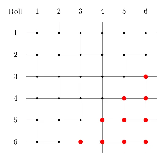
Let be the event that the sum is greater than 8, and let be the event that the first roll is 4. Conditioning on restricts attention to the fourth column. The outcomes in are and .
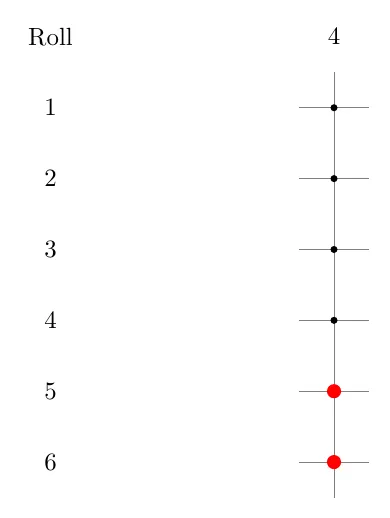
Then and , so
This is the same as counted inside the subspace .
Both readings are valid: one uses the original measure, the other counts directly in the compressed sample space. The second is easier when the subspace cannot be drawn.
With this example, I believe that you must know how conditional probability is all about. However, this is only a very special case. You may have noticed that for rolling a fair dice, we have equal possibility to get 1-6 in each roll. In the real life, most events have different probabilities. Let's see another example of unfaired dice. But to solve this problem, we need to use an important conclusion of conditional probability.
By multiplying to , we find that
An unfair four-sided die (numbered 1 to 4) is rolled twice. The biases for the die are:
We are tasked with calculating:
-
The conditional probability that the sum of the two rolls is 4, given that the first roll is a 2.
-
The conditional probability that the first roll is a 2, given that the sum of the two rolls is 4.
Define the events:
-
: The sum of the two rolls is 4.
-
: The first roll is a 2.
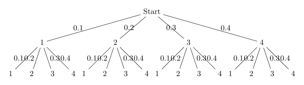
We can draw a tree diagram to show all possible results with the probability of each branch.
1.
The event fixes the first roll at 2. For to occur with , the second roll must be 2 (i.e., ).
This could also easily be examined from the graph the 2-2 is the only branch among the four possible cases under 2 in the first roll, so we have .
We get by using the corollary to the numerator, which is the probability of getting a two twice. By the corollary, it can be expressed as the product of the probability we get 2 in the second trial given that 2 is ontained in the first attempt, and . It is obvious that the condition does not work here, because we always have the same chance of getting a 2. Thus we have as the numerator of .
2.
The event (sum is 4) can occur through the following combinations:
-
and
-
Calculate :
Note that:
-
We use Eq intasprob here, since for some event , . We get the probability of each branch by using the RHS of the equation using the probability on the edge of the tree diagram. E.g., we have 3 for the second roll and 1 in the first roll, then we have chance for the coresponding result.
-
The weight on the tree graph in every layer are treated as conditional probability, and 0.3 is the probability of a three given that the first roll gives 1
-
Also notice that all branches are disjoint, so we use additibity axiom here to sum up the probability.
Now, :
From this example we see that despite that we have different probability for each branch of events, what we are doing to find conditional probability is still the same: subsetting the sample space and locate our target cases in that subspace.
We wrap up the use of lattice diagram and tree diagram here.
Lattice Diagram
Lattice diagrams are particularly useful for representing all possible outcomes in a sequence of events where outcomes are straightforward and often uniformly distributed, such as flipping coins or rolling dice. They are excellent for visualizing permutations, combinations, and the structure of outcomes in multi-stage experiments. A lattice diagram efficiently showcases how different paths can lead to various results, making it ideal for illustrating scenarios with equal probabilities or for modeling situations like financial derivatives pricing, where the path dependencies of options or other financial instruments are important.
Tree Diagram
Tree diagrams, on the other hand, excel in situations where outcomes have different probabilities(i.e., not uniformly distributed ) or the process is inherently hierarchical. They are invaluable for breaking down complex probability problems into manageable parts, especially in Bayesian statistics where updates to probability estimates are made as new information becomes available. Tree diagrams allow for the visualization of conditional probabilities and sequential decision processes, making them perfect for scenarios where events are dependent on previous outcomes, such as sequential games, Bayesian inference, or decision analysis.
But of course, we will not always use diagram for problem-solving, since you can imagine how complex the diagram could be when the scale of the problem increases. Fundamentally, we still need to obtain the result by analyzing the chain of events and their relations with the given conditions in different contexts.
Here are some more interesting examples.
Celine is undecided whether to take a French course or a chemistry course. She estimates that her probability of receiving an A grade would be in a French course and in a chemistry course. If Celine decides to base her decision on the flip of a fair coin, what is the probability that she gets an A in chemistry?
Let be the event that Celine takes the chemistry course and be the event that she receives an A in whatever course she takes. The decision to take chemistry is based on the flip of a fair coin, thus .
Given (the event of taking chemistry), the probability of (receiving an A) in chemistry is . Therefore, the probability that Celine takes chemistry and gets an A can be calculated using the rule of multiplication for probabilities:
Thus, the probability that Celine gets an A in chemistry, given that her decision is based on a coin flip, is .
Some people may wonder why we are calculating probability of intersection instead of conditional probability here. Because semantically, the probability of getting A in chemistry given that we get head/tail of the coin seems equivalent to the probability of getting A in chemistry, and we get head/tail of the coin. The answer if completely NO. Because when we gauge the conditional probability, condition(s) matters. Will the result of flipping the coin affact the chance of getting A in chemistry? Of course no, so we are not finding a conditional probability. We will discuss this further in independence of events. This is a vivid example that demonstrates the difference of sumbolic language and natural language. The former outperforms in terms of accuracy but less understandable for human, while natural language is more understandable but in many cases, bring a lot of bias.
Suppose that an urn contains 8 red balls and 4 white balls. We draw 2 balls from the urn without replacement.
(a) If we assume that at each draw, each ball in the urn is equally likely to be chosen, what is the probability that both balls drawn are red?
(b) Now suppose that the balls have different weights, with each red ball having weight and each white ball having weight . Suppose that the probability that a given ball in the urn is the next one selected is its weight divided by the sum of the weights of all balls currently in the urn. Now what is the probability that both balls are red?
(a) Let and denote, respectively, the events that the first and second balls drawn are red. Given that the first ball selected is red, there are 7 remaining red balls and 4 white balls, so . As is clearly , the desired probability is calculated as:
(b) For this part, we again let be the event that the -th ball chosen is red and use:
Now, number the red balls, and let be the event that the first ball drawn is red ball number . Then:
Moreover, given that the first ball is red, the urn then contains 7 red and 4 white balls. Thus, by a similar argument:
Hence, the probability that both balls are red is:
Now let's move further onto the generalization of corollary intersectascond, known as The multiplication rule of probability. Multiplication rule is used to calculate the probability of an event after a chain of event. In fact, we are using the previous definition multiple times here.
If are events, then the probability of all these events occurring in sequence is given by:
We prove the theorem by induction on the number of events .
Base case (): For two events and , the multiplication rule reduces to:
which is the definition of the conditional probability of given .
Inductive step: Assume that the theorem holds for events. That is, we assume:
We need to prove that the rule holds for events. By the definition of conditional probability, we have:
Applying the induction hypothesis, we substitute for :
which confirms the theorem for events.
Thus, by the principle of mathematical induction, the multiplication rule holds for any number of events.
Actually, we have a more decent way to prove it, which works like chain rule in differentiation.To prove the multiplication rule, just apply the definition of conditional probability to its right-hand side, giving
An ordinary deck of 52 playing cards is randomly divided into 4 piles of 13 cards each. Compute the probability that each pile has exactly 1 ace.
Define events , , as follows:
The desired probability is , and by the multiplication rule,
Now, since is the sample space . To determine , consider the pile that contains the ace of spades. Because its remaining 12 cards are equally likely to be any 12 of the remaining 51 cards, the probability that the ace of hearts is among them is , giving that
Also, given that the ace of spades and ace of hearts are in different piles, it follows that the set of the remaining 24 cards of these two piles is equally likely to be any set of 24 of the remaining 50 cards. As the probability that the ace of diamonds is one of these 24 is , we see that
Because the same logic as used in the preceding yields that
the probability that each pile has exactly 1 ace is
That is, there is approximately a 10.5 percent chance that each pile will contain an ace. (Problem 13 gives another way of using the multiplication rule to solve this problem.)
Exercises
The locked source file leaves this exercise heading empty. Developed exercises resume after Bayes's theorem.
Bayes's Theorem
Bayes's Theorem and Bayesian Thinking
We can do more with conditional probability. Now consider event and . Regardless of what kind of events they are, we always have
This makes sense not only from set theory's conclusion but also in terms of practicality. Because for any two events, assuming one of them will happen, then the other one could either happen or not happen. We know that are mutually exclusive, so by additivity axiom, we have
This can be interpreted as: the probability of the event E is measured by the weighted average of of the possibility that F happens and not happens. This formula enables us to get the probability of an event by conditioning the probability of some other events and its complement. This is very important for us, since some times we cannot get the probability of a certain event easily. The following example shows its advantage in finding conditional probability (in a reversed order).
An insurance company believes that people can be divided into two classes: those who are accident prone and those who are not. The company's statistics show that an accident-prone person will have an accident at some time within a fixed 1-year period with probability .4, whereas this probability decreases to .2 for a person who is not accident prone. If we assume that 30 percent of the population is accident prone, what is the probability that a new policyholder will have an accident within a year of purchasing a policy?
We shall obtain the desired probability by first conditioning upon whether or not the policyholder is accident prone. Let denote the event that the policyholder will have an accident within a year of purchasing the policy, and let denote the event that the policyholder is accident prone. Hence, the desired probability is given by
Note that in the previous example, we used the probability of given or . The next example shows how we can get the probability of given .
Suppose that a new policyholder has an accident within a year of purchasing a policy. What is the probability that he or she is accident prone?
The desired probability is
The figure uses an illustrative population of policyholders. Its event is the first-year accident event above. Filtering leaves people, so the accident-prone share becomes .
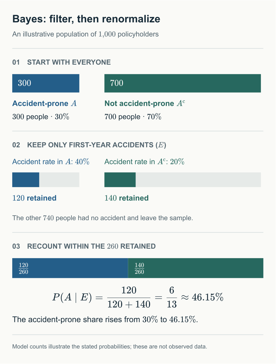
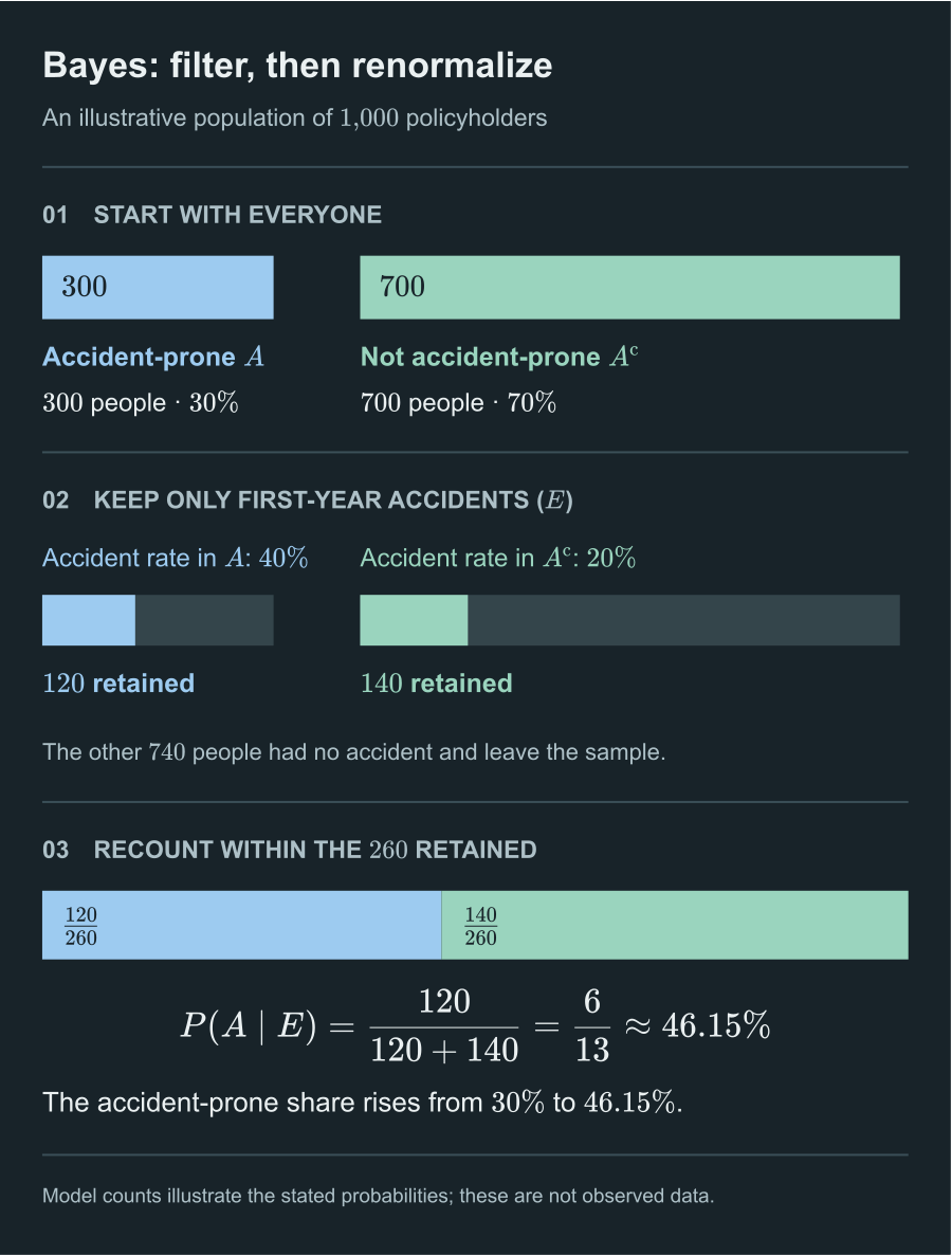
With this example, we have determined that knowing the probability of an event (in this case, we can obtain its complement using the complement rule such that ), given another event and its complement , enables us to calculate the probability of given .
This is known as Bayes's Theorem. The interesting part of the theorem lies not only in terms of algebra or practical significance, but it also illustrates a thinking pattern.
Given two events and , with , Bayes' theorem describes the probability of event given that event has occurred, and is formally defined as:
where:
-
is the posterior probability of event occurring given the occurrence of event .
-
is the likelihood, which is the probability of observing event given that event has occurred.
-
is the prior probability of event occurring.
-
is the marginal probability of event , which can also be calculated using the law of total probability if the complete set of outcomes related to is known:
Assume as well as so both displayed conditional probabilities are defined. The definition gives . Divide by . In a total-probability denominator, the must form a finite or countable disjoint partition; omit zero-probability cells before forming conditional terms. When , the posterior is directly zero by monotonicity, while is undefined under this elementary event definition.
The Bayes's Formula is extremely concise and easy to understand, however profound philosophical and cognitive significance are combined into this expression.
Bayes's formula models the way human make judgment, of course, in a wise way. For each term of the formula, we have given an definition, which we need to figure out.
-
The prior probability is the existing belief in a certain event.
-
The likelihood is an factor that helps people make further judgment, which means the possibility of something else to happen under some given facts(in someone's mind, but may not a 100% true fact).
-
The marginal probability refers to the possibility of the other related event.
-
Posterior Probability refers to the new possibility given some other event(s) that fix/update the prior probability to a reasonable level.
If I tell you, this is exactly how human-beings , not just as an individual, but a civilization, learn, you may confuse that these seem very elusive and abstract, but we can clarify this by using one example.
Consider asking the question that "Is the earth flat or a sphere" to someone randomly picked from somewhere in the world, almost everyone will say yes, out of common sense. But clearly people do not always think so. In the past, or more specifically, before human-beings grasp the way of examine and measuring the nature, most people believe that we live on a flat land. However, with the advance of sailing technique, thrive of colonialism, and a cascade of geographical discovery, some people slightly change their mind, finding some tiny possibility that we live on a sphere. Only until the first global circling sail is done, that the earth is a sphere becomes acceptable to more and more people and finally become a common sense.
In this example, the prior probability of the event that the earth of is flat decreases, while the possibility of the contradictory event that the earth of sphere increases. We can analyze the numerator and denominator of the formula, and we will find that approaches to 0 and approaches to 1. Eventually, this makes the probability that earth is flat given all new known facts(observation from ) to almost 0. This is exactly how we learn new things.
Though we know the interesting example, we still cannot prove it. We have shown how this makes sense previously, but only one thing is different here, since we consider that there could be any amount out comes for , while previously we used the base case where is a binary event, meaning it is only considered happen or not happen.
To work this problem out, we first introduces the law of total probability.
Let be a finite or countably infinite partition of the sample space , such that for all and , with for all . For any event in ,
Consider the event and the partition of the sample space . Since these sets are mutually exclusive and collectively exhaustive,
Because the sets are mutually exclusive,
Using the definition of conditional probability,
Thus,
which is the statement of the law of total probability.
You may also prove this by induction with as a base case using the conclusion of the beginning of the section.
Now we can proceed to prove Bayes's Theorem.
Proof of Bayes's Theorem. Assume is a partition of the sample space, and is any event in the sample space. According to the law of total probability, we have:
Using the definition of conditional probability, we express as:
Substituting this back into the law of total probability, we obtain:
Now, consider the conditional probability for some . By definition, it is:
Substituting into the equation, we get:
Since can be expanded using the law of total probability, it becomes:
This equation is Bayes' Theorem for the case where the partition consists of events. For the simpler case with only one and its complement , Bayes' Theorem simplifies to:
Here are some typical problems.
At a certain stage of a criminal investigation, the inspector in charge is convinced of the guilt of a certain suspect. Suppose, however, that a new piece of evidence which shows that the criminal has a certain characteristic (such as left-handedness, baldness, or brown hair) is uncovered. If of the population possesses this characteristic, how certain of the guilt of the suspect should the inspector now be if it turns out that the suspect has the characteristic?
Let denote the event that the suspect is guilty and the event that he possesses the characteristic of the criminal. We use Bayes' theorem to update our belief about given :
Applying the law of total probability to the denominator,
Given that and (since the suspect being not guilty is the complement of the suspect being guilty), and assuming (if the suspect is guilty, he definitely has the characteristic) and (the probability that a non-guilty person has the characteristic),
Thus,
This indicates that, given the suspect has the characteristic, the inspector should now be approximately certain of the suspect's guilt.
Suppose that we have 3 cards that are identical in form, except that both sides of the first card are colored red, both sides of the second card are colored black, and one side of the third card is colored red and the other side black. The 3 cards are mixed up in a hat, and 1 card is randomly selected and put down on the ground. If the upper side of the chosen card is colored red, what is the probability that the other side is also colored red?
Let , , and denote the selected card, and let mean that its upper side is red. Assume each card is equally likely and either side is equally likely to face up. Then
Given a red upper side, the lower side is red exactly when the card is . Since ,
Equivalently, the three possible red upper faces consist of two faces from and one from . Two of these three outcomes have a red lower face. The remaining probability is for a black lower face. The two possible card types are not equally likely after observing red.
Before applying conditional probability, specify how the observation is sampled. The next example depends on which child is selected to accompany the mother.
A new couple, known to have two children, has just moved into town. Suppose that the mother is encountered walking with one of her children. If this child is a girl, what is the probability that both children are girls?
Assume the children's sexes are independent and equally likely, and that either child is equally likely to accompany the mother, independently of sex. Under this sampling model, define:
-
: the first (that is, the oldest) child is a girl.
-
: the second child is a girl.
-
: the child seen with the mother is a girl.
Also, let and denote similar events, except that "girl" is replaced by "boy." Now, the desired probability is , which can be expressed as follows:
where can be calculated using the law of total probability:
Given that and and and , and assuming that all four gender combinations are equally likely ( each),
Now, is simply the probability of having two girls, which is , so
Therefore,
Thus, if the child seen is a girl, the probability that both children are girls is .
Independence of Events
Definition of Independence
previously, we defined the conditional probability of some event given by
You may recall that, in some examples earlier, we find , and we have . In this case, we claim that is independent of .
Two events E and F are said to be independent if and only if
Here's a basic example.
Suppose that we toss two fair dice. Consider the following events:
-
: The event that the sum of the dice is 6.
-
: The event that the first die equals 4.
We are interested in determining whether these two events are independent.
First, calculate and , and then to check for independence:
- The probability that the sum of the dice equals 6, , can happen through the combinations . Thus,
because there are 5 favorable outcomes out of 36 possible outcomes when two dice are thrown.
- The probability that the first die equals 4, , is simply,
since one out of six faces of a die shows 4.
- The probability of both and occurring, , happens only if the first die is 4 and the second die is 2 (to make the sum 6). Thus,
because there is only one favorable outcome for this combination under the condition that two dice are thrown.
Now, to check for independence, we examine if :
Clearly, , indicating that and are not independent.
Another fact about independent event is that if two events are independent to each other, then they are also independent of each other's complement event.
If and are independent, then so are and .
Assume that and are independent. Since can be expressed as the union of disjoint events and , we write
Using the independence of and , we have
Thus, the probability of can be rewritten using the complement rule as
Rearranging terms gives
Hence, shows that and are independent.
Multiple Independence
We have discussed the base case of independence between two events, how it is like for more events? Here is an example.
Two fair dice are thrown. Let denote the event that the sum of the dice is 7. Let denote the event that the first die equals 4 and denote the event that the second die equals 3. From earlier discussions, we know that is independent of , and the same reasoning shows that is also independent of . However, we find that is not independent of the joint event because . Given:
-
: Sum of two dice is 7.
-
: First die is 4.
-
: Second die is 3.
Independence Analysis:
- and are independent:
- and are independent:
- and are not independent. If and both occur, the sum is automatically 7, so
Then
Indeed, and , so
Thus, while is independent of both and individually, it is not independent of the joint event , illustrating how independence between individual events does not necessarily extend to independence with joint events.
Three events , , and are said to be independent if the following conditions hold:
Note that if , and are independent, then will be independent of any event formed from and For instance, is independent of ,since
You may find that this notion is kind of like inclusion-exclusion, and the only difference is that we are not taking the case of one object into account. We can easily extend the definition of independence to infinitely many events, which will be an exercise probelm.
Consider an infinite sequence of independent trials, each resulting in a success with probability and a failure with probability . Determine the probability that:
-
At least 1 success occurs in the first trials.
-
Exactly successes occur in the first trials.
-
All trials result in successes.
(a) Probability of at least one success in the first trials
To find this probability, it's easiest to first compute the probability of the complementary event: no successes in the first trials. If denotes a failure on the -th trial, by independence, the probability of no successes is:
Thus, the probability of at least one success is:
(b) Probability of exactly successes in the first trials
Consider any specific sequence of outcomes containing successes and failures. Each sequence occurs with probability , and the number of such sequences is given by the binomial coefficient :
(c) Probability that all trials result in successes By part (a), the probability that the first trials all result in success is . The event that all trials result in success is the intersection of the events of success on each trial, , over an infinite number of trials. Using the continuity property of probabilities:
This limit is 0 if and 1 if , reflecting that only if success is certain on every trial (i.e., ) will we surely have success on every trial in an infinite sequence.
Consider independent trials consisting of rolling a pair of fair dice. What is the probability that an outcome of 5 appears before an outcome of 7 when the outcome of a roll is the sum of the dice?
If we let denote the event that no 5 or 7 appears on the first trials and a 5 appears on the -th trial, then the desired probability is:
Given and , by the independence of trials, we compute:
Therefore, the probability is:
Alternative Method: The probability can also be derived using conditional probabilities:
Solving for , we get .
The answer is intuitive as the probability of a 5 occurring on any roll is and for a 7 is . Thus, the probability that a 5 appears before a 7 should be , as indeed it is.
if and are mutually exclusive events of an experiment, then, when independent trials of the experiment are performed, the event will occur before the event with probability
Exercises
Suppose rolling a fair dice twice, is the event that the sum of two trial is 7 independent of the first roll? Prove or disprove it. Explain the reason.
Let represent the event that the sum of the dice is 7, and the event that the first die shows . The events are independent if for each .
Calculation:
- The probability that the sum equals 7, , is the number of favorable outcomes over the total outcomes when rolling two dice:
- The probability of rolling any specific number on a fair die, , is:
- The probability of both and occurring simultaneously, , happens only when the first die is and the second die rolls . Thus:
Checking Independence: Since the product of and is:
and this is equal to , the equality:
holds for each , proving that and are independent. Knowing the outcome of the first die roll does not affect the probability of the sum being 7.
This conclusion follows from the fact that the condition required for depends equally on both dice, and the outcome of one does not skew the likelihood of achieving a total of 7 compared to any other total.
Use the definition below to show that each event is independent of every Boolean combination of the remaining events.
A set of events is said to be mutually independent if and only if for every nonempty subset of these events, the probability of the intersection of these events equals the product of their probabilities:
This must hold for every with and for every subset of indices .
Assume is a set of mutually independent events. We need to show that for any and for any event formed from using any Boolean operations, the events and are independent, i.e., .
Since can be expressed as a union of intersections of events and their complements from , we apply the principle of inclusion-exclusion and the mutual independence assumption:
Each term reduces to the product of probabilities of or by independence.
For , apply the same decomposition:
By mutual independence, each intersection involving simplifies to times the product of probabilities from the other events or their complements, verifying that:
Thus, is independent of any Boolean combination of the remaining events, as required.
Further Conditional Probability
Probability Axiom in Conditional Probability
In the previous sections we introduced conditional probability and Bayes's formula. The next step is to push those identities further so that more problems can be solved.
We introduced the three axioms of probability and many propositions derived from them. While conditional probability is also a kind of "special" probability, these rules should also work for them, but as usual, we must provide rigorous proof.
Let and be events, and let , for , be a sequence of mutually exclusive events. Then:
-
.
-
where is the sample space.
-
If , , are mutually exclusive, then
To prove part (a), note that since , it follows that , hence as . For part (b), since , we have . Part (c) follows from the properties of probability measures over countable unions of disjoint sets and the definition of conditional probability:
Conditioning therefore preserves the probability axioms.
If we define , then can be regarded as a probability function on the events of , and the propositions previously proved for probabilities apply to . For instance,
Fix . Nonnegativity, normalization, and countable additivity were proved immediately above, which are exactly the probability axioms for . For the displayed identity, multiply ordinary inclusion-exclusion for and by . Their intersection is , producing the stated conditional formula.
It means that all conclusions about probability that we have proven are applicable to conditional probability. Also, do check exercise 1 of this section before moving on to the next example.
Consider a scenario involving an insurance company that categorizes new policyholders into two groups: those who are accident prone and those who are not. It is known that:
-
The probability that an accident-prone person has an accident in any given year is 0.4.
-
The probability that a person who is not accident-prone has an accident in any given year is 0.2.
-
The proportion of the accident-prone population among new policyholders is .
Given that a new policyholder has had an accident in the first year of their policy, what is the probability that they will have another accident in the second year?
Let denote the event that the policyholder is accident-prone, and let and denote accidents in the first and second years. Assume that the policyholder's type stays fixed and that yearly accidents are conditionally independent given that type. The annual probabilities alone would not determine the answer without a dependence assumption.
From the first-year accident, Bayes' rule gives
Conditional independence gives and . Therefore,
Let be mutually exclusive, exhaustive hypotheses. Assume the observed events have positive probability, and omit any zero-posterior hypotheses from conditional expressions.
After observing ,
The general update after observing retains in the new likelihood:
where
If and are conditionally independent given each hypothesis, the likelihood simplifies to . Then
The denominator is the joint evidence , a product rather than a ratio. For example, choose one coin of unknown identity from a collection with known biases, then flip that same coin repeatedly. Conditional on its identity, independent flips let us update using the current posterior and the next likelihood, without storing every earlier outcome separately.
Multi-conditional Probability
We can also generalize conditional event with multiple conditions. All we need to do is taking the intersection of the rest of the conditions(except one of the condition), as a single event. This could be proven easily with mathematical induction.
The multi-conditional probability of an event given multiple events is defined by the formula:
provided that .
Set . When , ordinary conditional probability gives
This is an application of the definition to an intersection, so no induction argument is needed. The events need not be independent.
A computer system's reliability is critical to an organization. The failure of this system can be influenced by multiple factors, some of which are interdependent. These factors include software malfunction (S), hardware malfunction (H), network failure (N), power surges (P), and user error (U).
-
-
-
-
-
(Conditional probability reflecting the likelihood of power surges and user error given the first three conditions)
Assess the comprehensive probability of system failure incorporating all these factors, taking into account their conditional dependencies.
First, calculate the joint probability of all factors:
Then, apply the multi-conditional probability:
Therefore, the comprehensive probability of system failure given all factors are:
Exercises
Show that proposition ex
holds and thus prove thatTo show that is a probability measure, we must verify that it satisfies the axioms of probability. Since and is a probability measure:
-
, since .
-
for any event , as conditional probabilities are non-negative.
-
For any sequence of mutually exclusive events ,
by the sigma additivity of and the definition of conditional probability.
Thus, behaves as a probability measure on , and by the properties of probability measures, the formula for the union of two events follows.
For the second part, assume and . The conditional probability under is
We can get the total probability of by
We also have
Similarly, .
Substituting, we have
If a branch has zero probability under , omit it; no conditional probability on a null event is needed. This completes the proof.
Comments