Matrix as Graph: Connections, Flows, and Transitions

One graph can support different matrices

A traffic graph asks whether flow balances. A webpage graph asks where a jump can lead. Both have vertices and directed edges, but they call for different matrix representations.

We first establish the graph-to-matrix correspondence, then use traffic and webpage transitions to see why different questions require different representations of a network [1][1] X. Yang, “ENG1005 Week 2: Traffic Flow, Personal Workshop Solutions,” 2024. Personal solutions to Monash ENG1005 workshop problems; source snapshot 77ebe58de2fea53d62533d6dd23caa16108ed109. Repository access may be restricted.. https://github.com/Eryc123Y/ENG1005-2024S2/blob/77ebe58de2fea53d62533d6dd23caa16108ed109/Source%20Code/W2.tex, [2][2] X. Yang, “ENG1005 Week 4: Webpage Transitions, Personal Workshop Solutions,” 2024. Personal solutions to Monash ENG1005 workshop problems; source snapshot 77ebe58de2fea53d62533d6dd23caa16108ed109. Repository access may be restricted.. https://github.com/Eryc123Y/ENG1005-2024S2/blob/77ebe58de2fea53d62533d6dd23caa16108ed109/Source%20Code/W4.tex. Prerequisites are matrix multiplication and linear systems.

Fix the graph’s meaning before writing its matrix

A finite directed graph consists of a vertex set $V$ and an edge set $E$. An edge $u\to v$ has a source and a destination. Our adjacency examples have no parallel edges between an ordered pair of vertices, although a model may include self-loops. With parallel edges, entries must count edges or sum their weights rather than remain binary.

A walk follows consecutive edges and may repeat vertices or edges; a simple path does not repeat vertices. Length counts edges traversed. A length-zero walk stays at its starting vertex, matching $A^0=I$.

An undirected edge appears in two symmetric adjacency positions. Thus an undirected loop-free graph has a symmetric adjacency matrix with zero diagonal. In a directed graph, having both directions available does not require equal weights.

Weights may represent flow, connection strength, distance, or probability. Ordinary multiplication does not interpret these units automatically. Path distance normally adds edge lengths and shortest paths minimize over alternatives; products of edge weights from ordinary matrix multiplication are not shortest-path lengths.

Adjacency records one-step connections

Fix a vertex order and use columns for sources, rows for destinations. For an unweighted directed graph, define

$$A_{ij}=\begin{cases} 1,&\text{if there is an edge }j\to i,\\ 0,&\text{otherwise}. \end{cases}$$

This convention suits multiplication of state columns: column $j$ records destinations from $j$. Some texts use the opposite convention, so check before calculating.

For vertices $A,B,C$ and edges $A\to B,A\to C,B\to C$,

$$A=\begin{pmatrix}0&0&0\\1&0&0\\1&1&0\end{pmatrix},\qquad A^2=\begin{pmatrix}0&0&0\\0&0&0\\1&0&0\end{pmatrix}.$$

There is one length-two walk from $A$ to $C$, through $B$.

PropositionPowers count walks

Under this convention, $(A^k)_{ij}$ counts walks of length exactly $k$ from $j$ to $i$. A walk may repeat vertices and edges; it need not be a simple path.

Proof

The case $k=1$ is the definition. Assuming the result for $k$,

$$(A^{k+1})_{ij}=\sum_\ell A_{i\ell}(A^k)_{\ell j}.$$

Each length-$(k+1)$ walk has a unique penultimate vertex $\ell$. Count its first $k$ steps from $j$ to $\ell$, then its last edge to $i$. Summing over $\ell$ counts every walk exactly once.

With weighted adjacency, powers instead sum the products of edge weights along walks.

Degree, weight, and probability

Under the source-column convention, column $j$ of an unweighted adjacency matrix sums to vertex $j$‘s outdegree, while row $i$ sums to vertex $i$‘s indegree. A self-loop contributes once to each.

For weighted graphs, these sums give total outgoing and incoming weight, often called strength, not necessarily edge counts. Two outgoing edges with weights $100,200$ give outdegree two and outgoing strength $300$.

If weights are probabilities, outgoing weight must sum to one for each source. If weights represent traffic, columns generally need neither normalization nor equal totals. Nonnegative entries alone do not make a matrix a transition matrix.

Transposition, relabelling, and isomorphism

With the convention fixed, $A^{\mathsf T}$ reverses all directed edges. The resulting graph need not be isomorphic to the original.

For a counterexample, take only $A\to B,A\to C$. The original has a vertex of outdegree two; the reversed graph has none. Relabelling cannot change that distinction.

Relabelling uses a permutation matrix. If old coordinates $\mathbf x$ become $\mathbf x'=P\mathbf x$, the new matrix is

$$A'=PAP^{-1}=PAP^{\mathsf T},$$

because $P(A\mathbf x)=A'\mathbf x'$. Rows and columns must be permuted together to preserve both endpoints of every edge. A third situation is changing the storage convention from source rows to source columns: the array is transposed, but the graph is unchanged because the interpretation also changes. These are different operations.

Relabelling the example explicitly

Change the three-vertex order from $(A,B,C)$ to $(B,A,C)$ with

$$P=\begin{pmatrix}0&1&0\\1&0&0\\0&0&1\end{pmatrix}.$$

The original edge $A\to B$ now goes from vertex two to vertex one. Relabelling every endpoint gives

$$PAP^{\mathsf T}=\begin{pmatrix}0&1&0\\0&0&0\\1&1&0\end{pmatrix}.$$

Connections are unchanged; their array positions change. Swapping only rows changes destination labels without making the same adjustment to sources, generally producing another graph.

Incidence records each edge’s balance

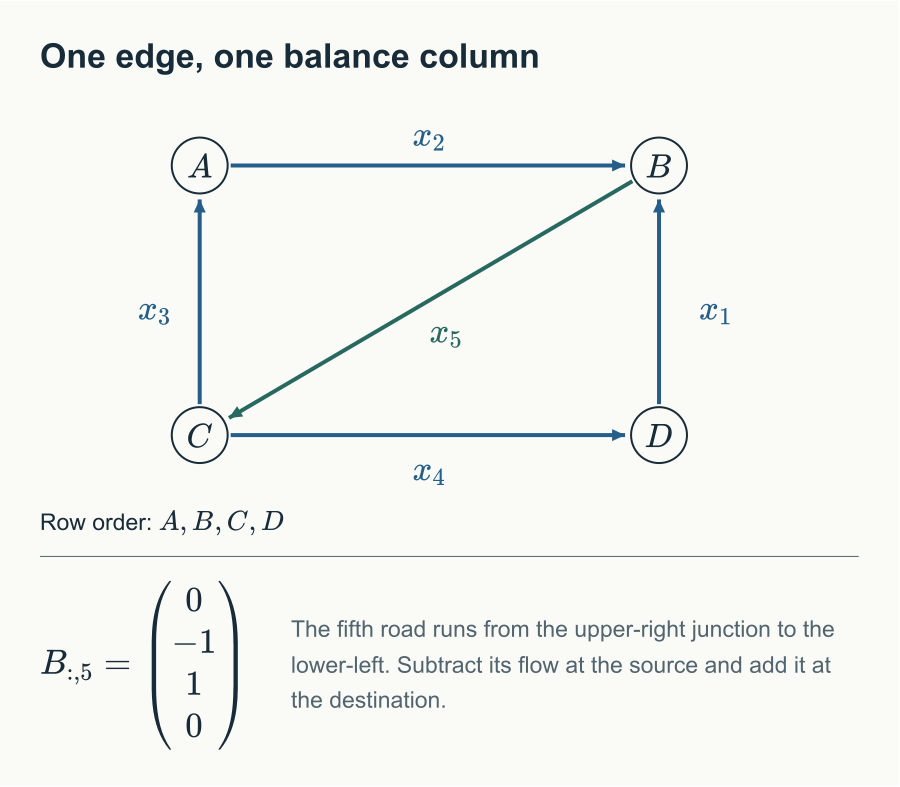
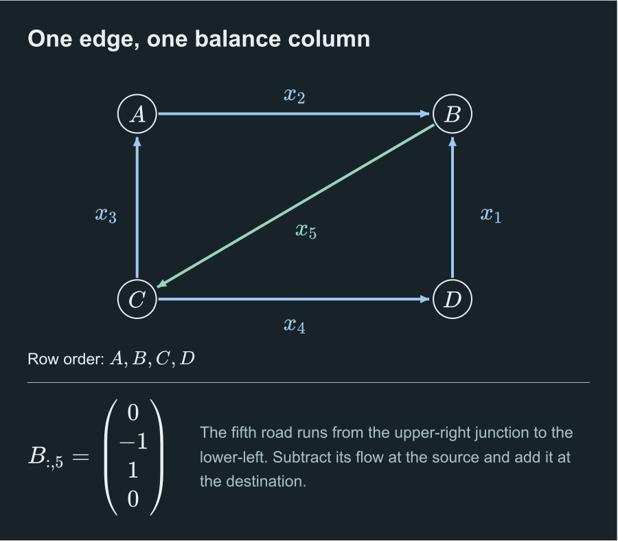
Return to the traffic network. Order rows as $A,B,C,D$ and columns as roads $x_1,\ldots,x_5$. A directed edge contributes $-1$ at its source and $+1$ at its destination:

$$B=\begin{pmatrix} 0&-1&1&0&0\\ 1&1&0&0&-1\\ 0&0&-1&-1&1\\ -1&0&0&1&0 \end{pmatrix}.$$

Adjacency has vertices on both axes; incidence has vertices on one axis and edges on the other. The product $B\mathbf x$ gives internal inflow minus internal outflow at each vertex. It must equal net external outflow:

$$B\mathbf x=\begin{pmatrix}-10\\45\\-45\\10\end{pmatrix}.$$

These are the equations from the systems chapter, with rows reordered and some signs reversed.

Every column has one $+1$ and one $-1$, so

$$\mathbf1^{\mathsf T}B=0.$$

Consequently, the right-hand side must sum to zero. Internal roads cannot create net inflow to the region.

Why four vertices give three independent balances

If $\mathbf z^{\mathsf T}B=0$, then each edge equates the $z$ values at its endpoints. When the underlying undirected graph is connected, all vertex values must agree. Thus every row dependence is a multiple of the sum relation, and the four rows have rank three.

More generally, an incidence matrix on $n$ vertices with $c$ connected components has rank $n-c$: the values of $z$ may be independently constant on each component. Connectivity here always ignores edge orientation.

Null directions describe circulations

The traffic model’s free directions are

$$\mathbf v_1=(1,-1,-1,1,0)^{\mathsf T},\qquad \mathbf v_2=(0,1,1,0,1)^{\mathsf T}.$$

The second adds equal flow around $A\to B\to C\to A$, cancelling at each vertex. The first also balances, but its negative components reduce flow relative to the road arrows. The nullspace therefore describes signed circulation changes, not necessarily physically admissible nonnegative traffic by themselves.

With five edges, four vertices, and a connected underlying graph, these changes have dimension $5-(4-1)=2$, matching elimination’s two free parameters.

Webpage transitions turn weights into probabilities

Consider random jumps between three webpages, described by

$$P=\frac1{10}\begin{pmatrix}2&1&3\\4&5&3\\4&4&4\end{pmatrix}.$$

Again, columns are sources and rows are destinations. Column one gives probabilities $0.2,0.4,0.4$ of reaching pages one, two, and three from page one. Each column is nonnegative and sums to one.

If $\mathbf x_n$ records expected page populations after step $n$, then

$$\mathbf x_{n+1}=P\mathbf x_n,\qquad \mathbf x_n=P^n\mathbf x_0.$$

Actual counts in a finite population fluctuate under random jumps; the matrix predicts expectations. Normalizing the state to a probability distribution gives the same equation.

Column sums preserve total population:

$$\mathbf1^{\mathsf T}P=\mathbf1^{\mathsf T} \quad\Longrightarrow\quad \mathbf1^{\mathsf T}\mathbf x_{n+1}=\mathbf1^{\mathsf T}\mathbf x_n.$$

Starting from $\mathbf x_0=(1000,1000,1000)^{\mathsf T}$ gives $(600,1200,1200)^{\mathsf T}$ after one step and $(600,1200,1200)^{\mathsf T}$ after three.

A stationary distribution satisfies

$$P\boldsymbol\pi=\boldsymbol\pi,\qquad \mathbf1^{\mathsf T}\boldsymbol\pi=1.$$

For this model,

$$\boldsymbol\pi=\frac15(1,2,2)^{\mathsf T},$$

as direct multiplication verifies. This is an eigenvector for eigenvalue $1$, but having a stationary distribution does not by itself prove convergence from every initial state. A matrix that swaps two vertices has stationary distribution $(1/2,1/2)^{\mathsf T}$, yet the state $(1,0)^{\mathsf T}$ oscillates forever. Below we prove convergence for the current model directly from its particular structure.

Turning nonnegative weights into probabilities

If column $j$ of a weighted adjacency matrix $W$ has sum $s_j>0$, normalize by source:

$$P_{ij}=\frac{W_{ij}}{s_j}.$$

This models choosing an outgoing edge proportionally to its weight. It is an additional assumption: if weights are road lengths, this rule favors longer roads and may not describe the desired behavior.

An all-zero column has no specified destination and cannot be normalized by division. The model must decide what happens, such as staying at the same vertex or restarting from a specified distribution. Different choices produce different transition matrices.

Why expected populations multiply by the matrix

If page $j$ currently has $x_j$ people and each has probability $P_{ij}$ of moving to page $i$, its expected contribution is $P_{ij}x_j$. Summing over source pages gives

$$\mathbb E[X_{n+1,i}\mid\mathbf X_n=\mathbf x] =\sum_jP_{ij}x_j.$$

This first conditions on current counts. If those counts are random too, taking expectation with the same fixed transition rule yields $\mathbb E[\mathbf X_{n+1}]=P\mathbb E[\mathbf X_n]$. Additivity of expectation does not require different people’s jumps to be independent; dependence affects fluctuations but does not invalidate this expectation formula.

Proving convergence for this particular matrix

Let total population be $N$, with expected page populations $g_n,h_n,m_n$. The third row gives

$$m_{n+1}=0.4(g_n+h_n+m_n)=0.4N.$$

After one step, the third component is fixed. Substitute $h_n=N-g_n-m_n$ into the first row. For $n\ge1$,

$$\begin{aligned} g_{n+1}&=0.2g_n+0.1h_n+0.3m_n\\ &=0.1g_n+0.1N+0.2m_n\\ &=0.1g_n+0.18N. \end{aligned}$$

Its fixed value satisfies $g_*=0.1g_*+0.18N$, giving $g_*=0.2N$. Subtracting that value reveals

$$g_{n+1}-0.2N=0.1(g_n-0.2N).$$

For $n\ge1$, induction gives

$$g_n-0.2N=0.1^{n-1}(g_1-0.2N).$$

The deviation tends to zero. Conservation determines the remaining component, proving convergence from every initial population distribution to $N(0.2,0.4,0.4)^{\mathsf T}$.

Starting from $(0,3000,0)^{\mathsf T}$ gives $(300,1500,1200)^{\mathsf T}$ and then $(570,1230,1200)^{\mathsf T}$. The first component’s deviation from $600$ shrinks from $-300$ to $-30$. Starting with $1000$ people per page lands exactly at stationarity after one step, a special initial condition rather than a general one-step convergence rule.

This proof uses the particular third row. General transition matrices need not simplify this way, and unit column sums alone do not imply convergence.

The same multiplication answers different questions

Representation	Meaning of a column	What multiplication describes
Adjacency	Edges leaving a vertex	Connections and walks
Incidence	One edge’s endpoint balance	Conservation and circulations
Transition	Destination probabilities from a vertex	Random state evolution

Before choosing a matrix, identify where the state lives, what each entry means, and which orientation convention applies.

Exercises

ExerciseTransitions need not be symmetric

What are the probabilities of moving from page one to page two and from page two to page one? Why may they differ?

Solution

They are $P_{21}=0.4$ and $P_{12}=0.1$. They condition on different source pages. Unit column sums do not require symmetry.

ExerciseCheck a circulation

Compute $B\mathbf v_2$. If $\mathbf x$ is feasible, is $\mathbf x+t\mathbf v_2$ feasible for every real $t$?

Solution

The product is zero, so all equality constraints remain satisfied. Negative $t$ may make some flows negative; physical feasibility still requires a componentwise check.

ExerciseWalks are not simple paths

Two vertices have one edge in each direction and no self-loops. Count length-two walks and explain why they need not be simple paths.

Solution

The adjacency matrix swaps coordinates, so its square is identity. Each vertex has one two-step return walk; there are no two-step walks between distinct vertices. Returning to the start repeats a vertex, so it is not a simple path.

ExercisePredicting through deviations

The three-page model has first-step state $(300,1500,1200)^{\mathsf T}$. Find its third-step state without a full matrix product.

Solution

The total is $3000$. The first component’s deviation from $600$ is multiplied by $0.1$ each step, giving deviation $-3$ at step three. The third component remains $1200$, so conservation gives state $(597,1203,1200)^{\mathsf T}.

References

1. [1] X. Yang, “ENG1005 Week 2: Traffic Flow, Personal Workshop Solutions,” 2024. Personal solutions to Monash ENG1005 workshop problems; source snapshot 77ebe58de2fea53d62533d6dd23caa16108ed109. Repository access may be restricted.. https://github.com/Eryc123Y/ENG1005-2024S2/blob/77ebe58de2fea53d62533d6dd23caa16108ed109/Source%20Code/W2.tex ↩
2. [2] X. Yang, “ENG1005 Week 4: Webpage Transitions, Personal Workshop Solutions,” 2024. Personal solutions to Monash ENG1005 workshop problems; source snapshot 77ebe58de2fea53d62533d6dd23caa16108ed109. Repository access may be restricted.. https://github.com/Eryc123Y/ENG1005-2024S2/blob/77ebe58de2fea53d62533d6dd23caa16108ed109/Source%20Code/W4.tex ↩